Understanding photothermal interactions can help expand production range and increase genetic diversity of lentil (Lens culinaris Medik.)
Plants, People, Planet. (2021) 3(2): 171-181.
Introduction
This vignette contains the code and analysis done for the paper:
- Derek M. Wright, Sandesh Neupane, Taryn Heidecker, Teketel A. Haile, Crystal Chan, Clarice J. Coyne, Rebecca J. McGee, Sripada Udupa, Fatima Henkrar, Eleonora Barilli, Diego Rubiales, Tania Gioia, Giuseppina Logozzo, Stefania Marzario, Reena Mehra, Ashutosh Sarker, Rajeev Dhakal, Babul Anwar, Debashish Sarker, Albert Vandenberg & Kirstin E. Bett. Understanding photothermal interactions can help expand production range and increase genetic diversity of lentil (Lens culinaris Medik.). Plants, People, Planet. (2021) 3(2): 171-181. doi.org/10.1002/ppp3.10158
- https://github.com/derekmichaelwright/AGILE_LDP_Phenology
This work done as part of the AGILE project at the University of Saskatchewan.

Data Preparation
Load the nessesary R packages, Prepare the data for analysis.
#install.packages(c("tidyverse","scales","rworldmap","ggrepel","magick",
#                   "GGally","ggpubr,"ggbeeswarm","FactoMineR","plot3D","stringr",
#                   "plotly","leaflet","leaflet.minicharts","htmlwidgets"))
# Load libraries
library(tidyverse)   # data wrangling
library(scales)      # rescale()
library(rworldmap)   # mapBubbles()
library(ggrepel)     # geom_text_repel() + geom_label_repel()
library(magick)      # image editing
library(GGally)      # ggpairs() + ggmatrix()
library(ggpubr)      # ggarrange()
library(ggbeeswarm)  # geom_quasirandom()
library(FactoMineR)  # PCA() & HCPC()
library(plot3D)      # 3D plots
library(stringr)     # str_pad()
library(plotly)      # plot_ly()
library(leaflet)     # leaflet()
library(leaflet.minicharts) # addMinicharts()
library(htmlwidgets) # saveWidget()
# General color palettes
colors <- c("darkred",   "darkorange3", "darkgoldenrod2", "deeppink3",
            "steelblue", "darkorchid4", "cornsilk4",      "darkgreen")
# Expts color palette
colors_Expt <- c("lightgreen",      "palegreen4",       "darkgreen",   "darkolivegreen3",
                 "darkolivegreen4", "springgreen4",     "orangered2",  "orangered4",
                 "palevioletred",    "mediumvioletred", "orange2",     "orange4",
                 "slateblue1",       "slateblue4",      "aquamarine3", "aquamarine4",
                 "deepskyblue3",     "deepskyblue4" )
# Locations
names_Location <- c("Rosthern, Canada", "Sutherland, Canada",  "Central Ferry, USA",
                    "Bhopal, India",    "Jessore, Bangladesh", "Bardiya, Nepal",
                    "Cordoba, Spain",   "Marchouch, Morocco",  "Metaponto, Italy" )
# Experiments
names_Expt <- c("Rosthern, Canada 2016",    "Rosthern, Canada 2017",
                "Sutherland, Canada 2016",  "Sutherland, Canada 2017",
                "Sutherland, Canada 2018",  "Central Ferry, USA 2018",
                "Bhopal, India 2016",       "Bhopal, India 2017",
                "Jessore, Bangladesh 2016", "Jessore, Bangladesh 2017",
                "Bardiya, Nepal 2016",      "Bardiya, Nepal 2017",
                "Cordoba, Spain 2016",      "Cordoba, Spain 2017",
                "Marchouch, Morocco 2016",  "Marchouch, Morocco 2017",
                "Metaponto, Italy 2016",    "Metaponto, Italy 2017" )
# Experiment short names
names_ExptShort <- c("Ro16", "Ro17", "Su16", "Su17", "Su18", "Us18",
                     "In16", "In17", "Ba16", "Ba17", "Ne16", "Ne17",
                     "Sp16", "Sp17", "Mo16", "Mo17", "It16", "It17" )
# Macro-Environments
names_MacroEnvs <- c("Temperate", "South Asia", "Mediterranean")
# Lentil Diversity Panel metadata
ldp <- read.csv("data/data_ldp.csv")
# Country info
ct <- read.csv("data/data_countries.csv") %>% filter(Country %in% ldp$Origin)
# ggplot theme
theme_AGL <- theme_bw() +
  theme(strip.background   = element_rect(colour = "black", fill = NA, size = 0.5),
        panel.background   = element_rect(colour = "black", fill = NA, size = 0.5),
        panel.border       = element_rect(colour = "black", size = 0.5),
        panel.grid         = element_line(color  = alpha("black", 0.1), size = 0.5),
        panel.grid.minor.x = element_blank(),
        panel.grid.minor.y = element_blank())
# Create scaling function
traitScale <- function(x, trait) {
  xout <- rep(NA, nrow(x))
  for(i in unique(x$Expt)) {
    mn <- x %>% filter(Expt == i) %>% pull(trait) %>% min(na.rm = T)
    mx <- x %>% filter(Expt == i) %>% pull(trait) %>% max(na.rm = T)
    xout <- ifelse(x$Expt == i, rescale(x %>% pull(trait), c(1,5), c(mn,mx)), xout)
  }
  xout
}
# Prep data
# Notes:
# - DTF2 = non-flowering genotypes <- group_by(Expt) %>% max(DTF)
rr <- read.csv("data/data_raw.csv") %>%
  mutate(Rep          = factor(Rep),
         Year         = factor(Year),
         PlantingDate = as.Date(PlantingDate),
         Location     = factor(Location, levels = names_Location),
         Expt         = factor(Expt,     levels = names_Expt),
         ExptShort    = plyr::mapvalues(Expt, names_Expt, names_ExptShort),
         ExptShort    = factor(ExptShort, levels = names_ExptShort),
         DTF2_scaled  = traitScale(., "DTF2"),
         RDTF         = round(1 / DTF2, 6),
         VEG          = DTF - DTE,
         REP          = DTM - DTF)
# Average raw data
dd <- rr %>%
  group_by(Entry, Name, Expt, ExptShort, Location, Year) %>%
  summarise_at(vars(DTE, DTF, DTS, DTM, VEG, REP, RDTF, DTF2),
               funs(mean), na.rm = T) %>%
  ungroup() %>%
  mutate(DTF2_scaled = traitScale(., "DTF2"))
# Prep environmental data
ee <- read.csv("data/data_env.csv") %>%
  mutate(Date      = as.Date(Date),
         ExptShort = plyr::mapvalues(Expt, names_Expt, names_ExptShort),
         ExptShort = factor(ExptShort, levels = names_ExptShort),
         Expt      = factor(Expt,      levels = names_Expt),
         Location  = factor(Location,  levels = names_Location),
         MacroEnv  = factor(MacroEnv,  levels = names_MacroEnvs),
         DayLength_rescaled = rescale(DayLength, to = c(0, 40)) )
# Prep field trial info
xx <- dd %>% group_by(Expt) %>%
  summarise_at(vars(DTE, DTF, DTS, DTM), funs(min, mean, max), na.rm = T) %>%
  ungroup()
ff <- read.csv("data/data_info.csv") %>%
  mutate(Start = as.Date(Start) ) %>%
  left_join(xx, by = "Expt")
for(i in unique(ee$Expt)) {
  ee <- ee %>%
    filter(Expt != i | (Expt == i & DaysAfterPlanting <= ff$DTM_max[ff$Expt == i]))
}
xx <- ee
for(i in unique(ee$Expt)) {
  xx <- xx %>%
    filter(Expt != i | (Expt == i & DaysAfterPlanting <= ff$DTF_max[ff$Expt == i]))
}
xx <- xx %>%
  group_by(Location, Year) %>%
  summarise(T_mean = mean(Temp_mean, na.rm = T), T_sd = sd(Temp_mean, na.rm = T),
            P_mean = mean(DayLength, na.rm = T), P_sd = sd(DayLength, na.rm = T) ) %>%
  ungroup() %>%
  mutate(Expt = paste(Location, Year)) %>%
  select(-Location, -Year)
ff <- ff %>%
  left_join(xx, by = "Expt") %>%
  mutate(ExptShort = plyr::mapvalues(Expt, names_Expt, names_ExptShort),
         ExptShort = factor(ExptShort, levels = names_ExptShort),
         Expt      = factor(Expt,      levels = names_Expt),
         Location  = factor(Location,  levels = names_Location),
         MacroEnv  = factor(MacroEnv,  levels = names_MacroEnvs),
         T_mean    = round(T_mean, 1),
P_mean = round(P_mean, 1))ldp= Lentil Diversity Panel Metadatarr= Raw Phenotype Datadd= Averaged Phenotype Dataee= Environmental Dataff= Field Trial Infoct= Country Info
Materials & Methods
Supplemental Table 1: LDP
Table S1: Genotype entry number, name, common synonyms, origin and source of lentil genotypes used in this study. These genotypes are gathered from the University of Saskatchewan (USASK), Plant Gene Resources of Canada (PGRC), United States Department of Agriculture (USDA), International Center for Agricultural Research in the Dry Areas (ICARDA).
s1 <- select(ldp, Entry, Name, Origin, Source, Synonyms)
write.csv(s1, "Supplemental_Table_01.csv", row.names = F)
Supplemental Table 2: Field Trial Info
Table S2: Details of the field trials used in this study, including location information, planting dates, mean temperature and photoperiods and details on plot type and number of seeds sown.
s2 <- ff %>%
  select(Location, Year, `Short Name`=ExptShort, Latitude=Lat, Longitude=Lon,
         `Planting Date`=Start, `Temperature (mean)`=T_mean, `Photoperiod (mean)`=P_mean,
         `Number of Seeds Sown`=Number_of_Seeds_Sown, `Plot Type`=Plot_Type)
write.csv(s2, "Supplemental_Table_02.csv", row.names = F)
xx <- ee %>%
select(ExptShort, Temp_min, Temp_max, DayLength) %>%
group_by(ExptShort) %>%
summarise(Temp_min = min(Temp_min),
Temp_max = max(Temp_max),
Photoperiod_min = min(DayLength),
Photoperiod_max = max(DayLength))
knitr::kable(xx)| ExptShort | Temp_min | Temp_max | Photoperiod_min | Photoperiod_max |
|---|---|---|---|---|
| Ro16 | -2.251 | 41.123 | 14.51 | 16.62 |
| Ro17 | 0.107 | 42.541 | 14.89 | 16.62 |
| Su16 | -3.720 | 46.528 | 14.51 | 16.52 |
| Su17 | -2.200 | 37.419 | 14.91 | 16.52 |
| Su18 | -0.686 | 41.940 | 13.94 | 16.52 |
| Us18 | 1.670 | 36.670 | 12.49 | 15.64 |
| In16 | 0.900 | 37.500 | 10.58 | 12.14 |
| In17 | 5.380 | 35.690 | 10.58 | 11.59 |
| Ba16 | 7.900 | 33.100 | 10.57 | 12.02 |
| Ba17 | 5.390 | 39.460 | 10.57 | 12.15 |
| Ne16 | 2.000 | 38.600 | 10.20 | 12.64 |
| Ne17 | NA | NA | 10.19 | 12.82 |
| Sp16 | -2.900 | 34.000 | 9.37 | 14.18 |
| Sp17 | -3.100 | 31.100 | 9.37 | 14.17 |
| Mo16 | -1.700 | 36.900 | 9.77 | 13.59 |
| Mo17 | -1.000 | 28.100 | 9.77 | 14.18 |
| It16 | -5.832 | 31.250 | 9.11 | 14.73 |
| It17 | -2.366 | 32.750 | 9.11 | 14.59 |
Figure 1: Field Trial Info
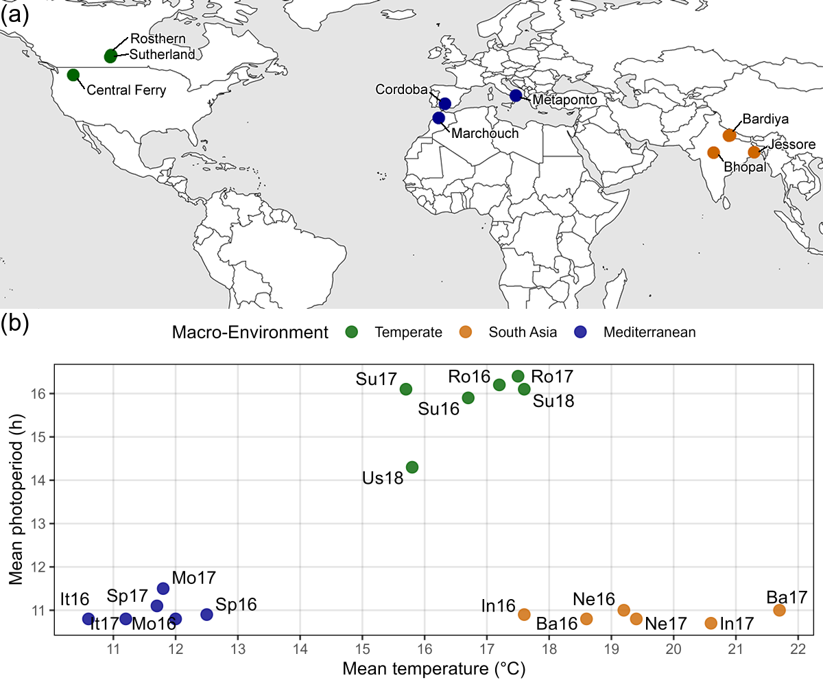
Figure 1: Growing Environments. (a) Locations of field trials conducted in the summer and winter of 2016, 2017 and 2018, along with (b) mean temperature and photoperiod of each field trial: Rosthern, Canada 2016 and 2017 (Ro16, Ro17), Sutherland, Canada 2016, 2017 and 2018 (Su16, Su17, Su18), Central Ferry, USA 2018 (Us18), Metaponto, Italy 2016 and 2017 (It16, It17), Marchouch, Morocco 2016 and 2017 (Mo16, Mo17), Cordoba, Spain 2016 and 2017 (Sp16, Sp17), Bhopal, India 2016 and 2017 (In16, In17), Jessore, Bangladesh 2016 and 2017 (Ba16, Ba17), Bardiya, Nepal 2016 and 2017 (Ne16, Ne17).
# Plot (a) Map
invisible(png("Additional/Temp/Temp_F01_1.png",
              width = 4200, height = 1575, res = 600))
par(mai = c(0,0,0,0), xaxs = "i", yaxs = "i")
mapBubbles(dF = ff, nameX = "Lon", nameY = "Lat",
           nameZColour = "MacroEnv", nameZSize = "Year",
           symbolSize = 0.5, pch = 20, fill = F, addLegend = F,
           colourPalette = c("darkgreen", "darkorange3", "darkblue"),
           addColourLegend = F,
           xlim = c(-140,110), ylim = c(10,35),
           oceanCol = "grey90", landCol = "white", borderCol = "black")
invisible(dev.off())
# Plot (b) mean T and P
mp <- ggplot(ff, aes(x = T_mean, y = P_mean)) +
  geom_point(aes(color = MacroEnv), size = 3, alpha = 0.8) +
  geom_text_repel(aes(label = ExptShort)) +
  scale_x_continuous(breaks = 11:22) + scale_y_continuous(breaks = 11:16) +
  scale_color_manual(name = "Macro-Environment",
                     values = c("darkgreen","darkorange3","darkblue")) +
  theme_AGL +
  theme(legend.position = "top", legend.margin = unit(c(0,0,0,0), "cm")) +
  labs(x = expression(paste("Mean temperature (", degree, "C)", sep = "")),
       y = "Mean photoperiod (h)")
ggsave("Additional/Temp/Temp_F01_2.png", mp,
       width = 7, height = 3.25, dpi = 600)
# Labels were added to "Additional/Temp/Temp_F1_1.png" in image editing software
# Append (a) and (b)
im1 <- image_read("Additional/Temp/Temp_F01_1_1.png") %>%
  image_annotate("(a)", size = 35)
im2 <- image_read("Additional/Temp/Temp_F01_2.png") %>%
  image_scale("1200x") %>%
  image_annotate("(b)", size = 35)
im <- image_append(c(im1, im2), stack = T)
image_write(im, "Figure_01.png")
Additional Figure 1: LDP Origin Map
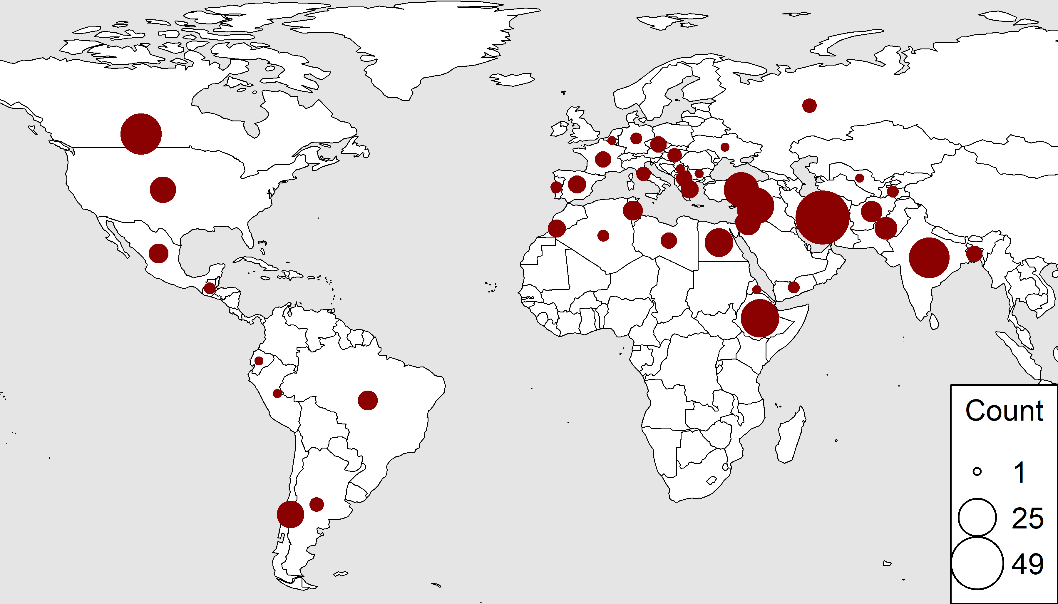
# Prep data
x1 <- ldp %>% filter(Origin != "Unknown") %>%
  mutate(Origin = recode(Origin, "ICARDA"="Syria", "USDA"="USA")) %>%
  group_by(Origin) %>%
  summarise(Count = n()) %>%
  left_join(select(ct, Origin = Country, Lat, Lon), by = "Origin") %>%
  ungroup() %>%
  as.data.frame()
x1[is.na(x1)] <- 0
# Plot
invisible(png("Additional/Additional_Figure_01.png",
              width = 3600, height = 2055, res = 600))
par(mai = c(0,0,0,0), xaxs = "i",yaxs = "i")
mapBubbles(dF = x1, nameX = "Lon", nameY = "Lat",
           nameZSize = "Count", nameZColour = "darkred",
           xlim = c(-140,110), ylim = c(5,20),
           oceanCol = "grey90", landCol = "white", borderCol = "black")
invisible(dev.off())
Supplemental Figure 1: DTF Scaling
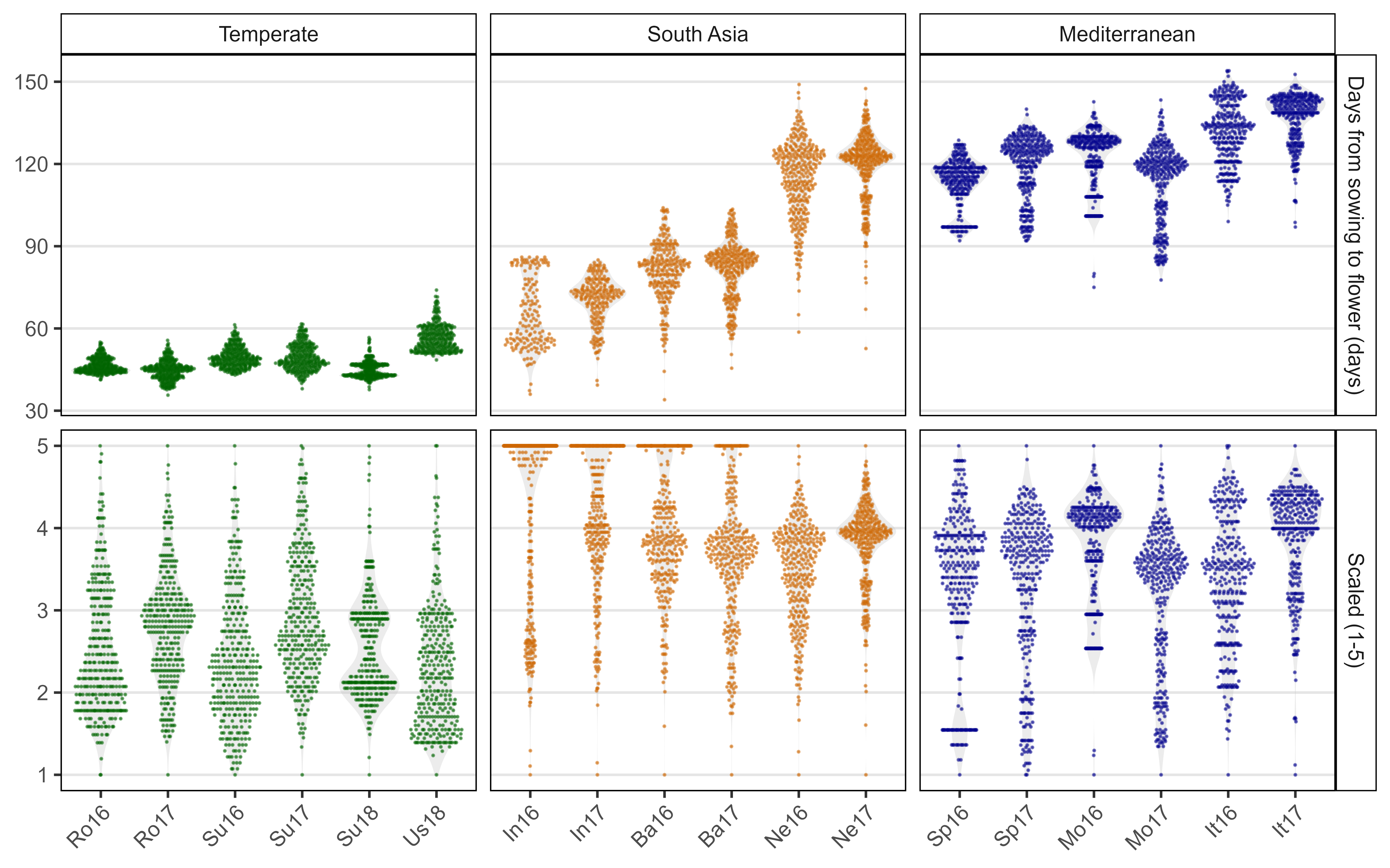
Figure S1: Distribution of days from sowing to flowering for raw data (top) and scaled data (1-5) (bottom) for all 18 field trials: Rosthern, Canada 2016 and 2017 (Ro16, Ro17), Sutherland, Canada 2016, 2017 and 2018 (Su16, Su17, Su18), Central Ferry, USA 2018 (Us18), Metaponto, Italy 2016 and 2017 (It16, It17), Marchouch, Morocco 2016 and 2017 (Mo16, Mo17), Cordoba, Spain 2016 and 2017 (Sp16, Sp17), Bhopal, India 2016 and 2017 (In16, In17), Jessore, Bangladesh 2016 and 2017 (Ba16, Ba17), Bardiya, Nepal 2016 and 2017 (Ne16, Ne17). Genotypes which did not flower were given a scaled value of 5.
# Prep data
levs <- c("Days from sowing to flower (days)", "Scaled (1-5)")
xx <- dd %>% select(Entry, Expt, ExptShort, DTF, DTF2_scaled) %>%
  left_join(select(ff, Expt, MacroEnv), by = "Expt") %>%
  gather(Trait, Value, DTF, DTF2_scaled) %>%
  mutate(Trait = plyr::mapvalues(Trait, c("DTF", "DTF2_scaled"), levs),
         Trait = factor(Trait, levels = levs) )
# Plot
mp <- ggplot(xx, aes(x = ExptShort, y = Value)) +
  geom_violin(fill = "grey", alpha = 0.3, color = NA) +
  geom_quasirandom(aes(color = MacroEnv), size = 0.1, alpha = 0.5) +
  scale_color_manual(values = c("darkgreen","darkorange3","darkblue")) +
  facet_grid(Trait ~ MacroEnv, scales = "free") +
  theme_AGL +
  theme(legend.position = "none",
        panel.grid.major.x = element_blank(),
        axis.text.x = element_text(angle = 45, hjust = 1)) +
  labs(x = NULL, y = NULL)
ggsave("Supplemental_Figure_01.png", mp, width = 8, height = 5, dpi = 600)
Phenology
Figure 2: Data Overview
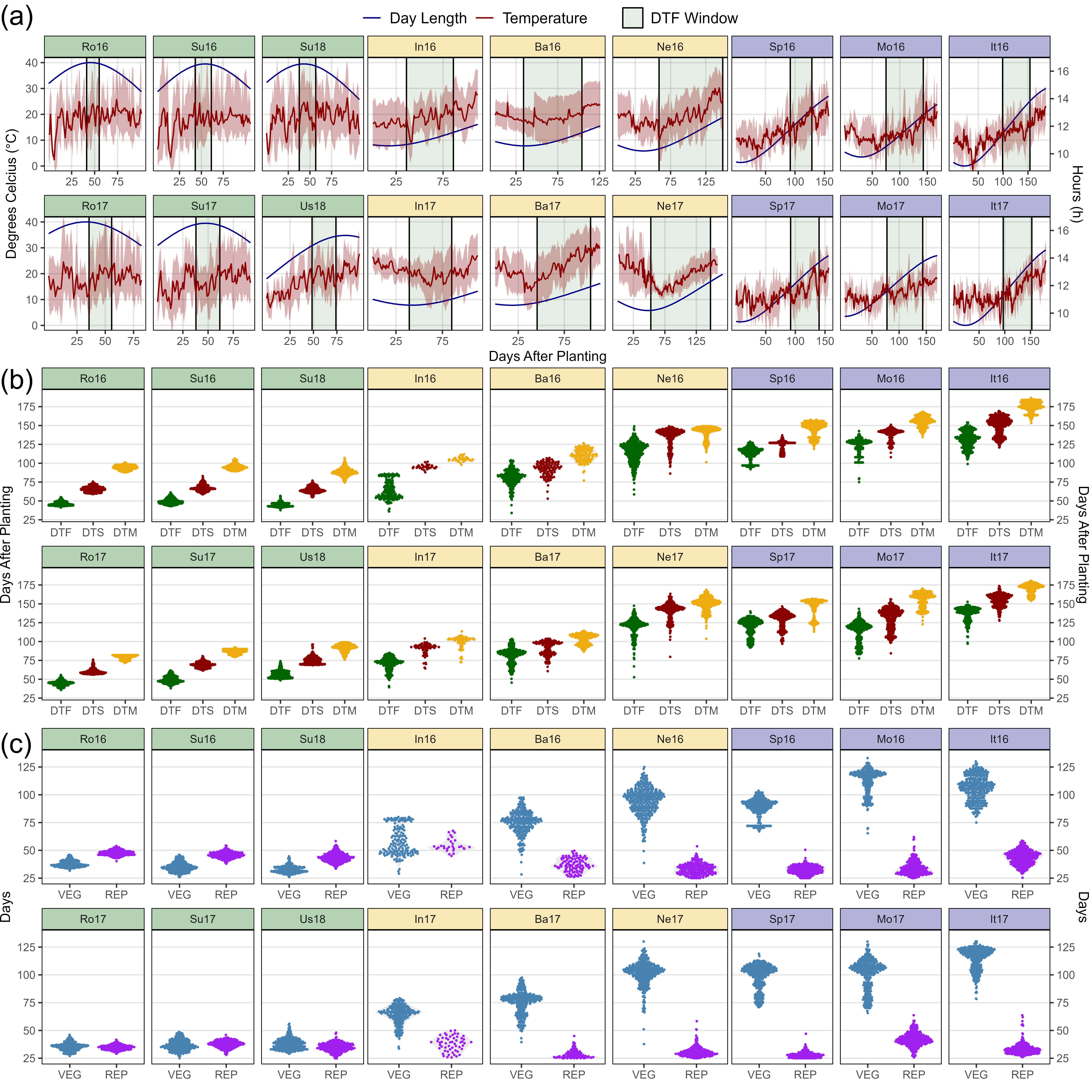
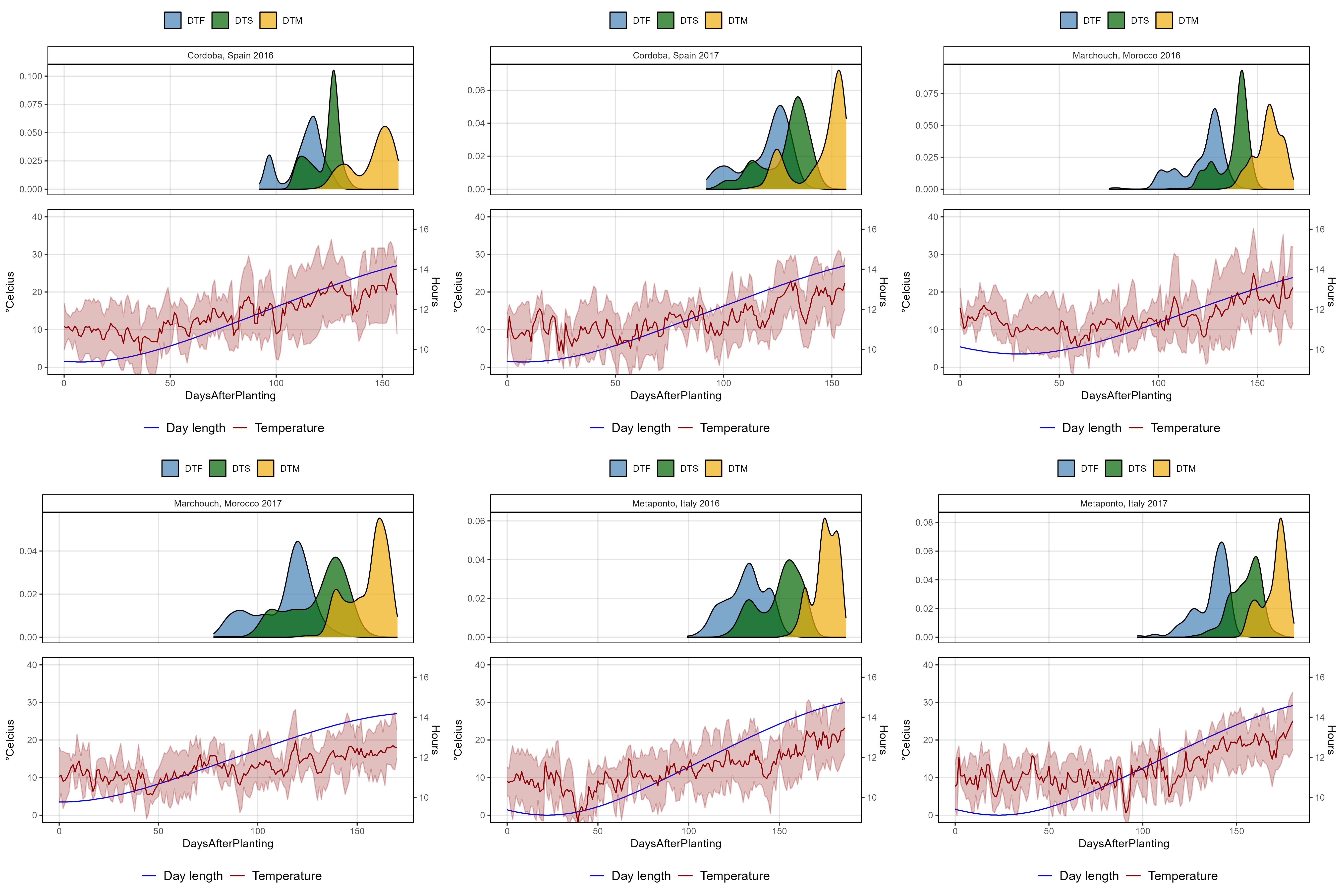
Figure 2: Variations in temperature, day length and phenological traits across contrasting environment for a lentil (Lens culinaris Medik.) diversity panel. (a) Daily mean temperature (red line) and day length (blue line) from seeding to full maturity of all genotypes. The shaded ribbon represents the daily minimum and maximum temperature. The shaded area between the vertical bars corresponds to the windows of flowering. (b) Distribution of mean days from sowing to: flowering (DTF), swollen pods (DTS) and maturity (DTM), and (c) vegetative (VEG) and reproductive periods (REP) of 324 genotypes across 18 site-years. Rosthern, Canada 2016 and 2017 (Ro16, Ro17), Sutherland, Canada 2016, 2017 and 2018 (Su16, Su17, Su18), Central Ferry, USA 2018 (Us18), Metaponto, Italy 2016 and 2017 (It16, It17), Marchouch, Morocco 2016 and 2017 (Mo16, Mo17), Cordoba, Spain 2016 and 2017 (Sp16, Sp17), Bhopal, India 2016 and 2017 (In16, In17), Jessore, Bangladesh 2016 and 2017 (Ba16, Ba17), Bardiya, Nepal 2016 and 2017 (Ne16, Ne17).
# Create plot function
ggEnvPlot <- function(x, mybreaks, nr = 2, nc = 3) {
  yy <- ff %>%
    filter(Expt %in% unique(x$Expt)) %>%
    select(ExptShort, Location, Year, min=DTF_min, max=DTF_max) %>%
    mutate(Trait = "DTF Window")
  ggplot(x) +
    geom_rect(data = yy, aes(xmin = min, xmax = max, fill = Trait),
              ymin = -Inf, ymax = Inf, alpha = 0.1, color = "black") +
    geom_line(aes(x = DaysAfterPlanting, y = DayLength_rescaled, color = "Day Length")) +
    geom_line(aes(x = DaysAfterPlanting, y = Temp_mean, color = "Temperature") ) +
    geom_ribbon(aes(x = DaysAfterPlanting, ymin = Temp_min, ymax = Temp_max),
                fill = "darkred", alpha = 0.3) +
    facet_wrap(ExptShort ~ ., scales = "free_x", dir = "v", nrow = 2, ncol = 3) +
    scale_x_continuous(breaks = mybreaks) +
    scale_color_manual(name = NULL, values = c("darkblue", "darkred")) +
    scale_fill_manual(name = NULL, values = "darkgreen") +
    guides(colour = guide_legend(order = 1, override.aes = list(size = 1.25)),
           fill = guide_legend(order = 2)) +
    coord_cartesian(ylim=c(0, 40)) +
    theme_AGL +
    theme(plot.margin = unit(c(0,0,0,0), "cm"),
          legend.text = element_text(size = 12)) +
    labs(y = NULL, x = NULL)
}
# Plot (a) T and P
mp1.1 <- ggEnvPlot(ee %>% filter(MacroEnv == "Temperate"), c(25, 50, 75)) +
  labs(y = expression(paste("Degrees Celcius (", degree, "C)"))) +
  theme(strip.background = element_rect(alpha("darkgreen", 0.3)),
        plot.margin = unit(c(0,0,0,0.155), "cm"))
mp1.2 <- ggEnvPlot(ee %>% filter(MacroEnv == "South Asia"), c(25, 75, 125)) +
  labs(x = "Days After Planting") +
  theme(strip.background = element_rect(fill = alpha("darkgoldenrod2", 0.3)),
        axis.text.y = element_blank(), axis.ticks.y = element_blank())
mp1.3 <- ggEnvPlot(ee %>% filter(MacroEnv == "Mediterranean"), c(50, 100, 150)) +
  scale_y_continuous(sec.axis = sec_axis(~ (16.62 - 9.11) * . / (40 - 0) + 9.11,
                     name = "Hours (h)", breaks = c(10, 12, 14, 16))) +
  theme(strip.background = element_rect(fill = alpha("darkblue", 0.3)),
        plot.margin = unit(c(0,0.17,0,0), "cm"),
        axis.text.y.left = element_blank(), axis.ticks.y.left = element_blank())
mp1 <- ggarrange(mp1.1, mp1.2, mp1.3, nrow = 1, ncol = 3, align = "h",
                 legend = "top", common.legend = T)
# Prep data
xx <- dd %>% select(Entry, Year, Expt, ExptShort, Location, DTF, DTS, DTM) %>%
  left_join(select(ff, Expt, MacroEnv), by = "Expt") %>%
  gather(Trait, Value, DTF, DTS, DTM) %>%
  mutate(Trait = factor(Trait, levels = c("DTF", "DTS", "DTM")))
# Create plot function
ggDistroDTF <- function(x) {
  ggplot(x, aes(x = Trait, y = Value) ) +
    geom_violin(color = NA, fill = "grey", alpha = 0.3) +
    geom_quasirandom(size = 0.3, aes(color = Trait)) +
    facet_wrap(ExptShort ~ ., scales = "free_x", dir = "v", ncol = 3, nrow = 2) +
    scale_color_manual(values = c("darkgreen", "darkred", "darkgoldenrod2")) +
    scale_y_continuous(limits = c(30,190), breaks = seq(25,175, 25)) +
    theme_AGL + labs(y = NULL, x = NULL) +
    theme(plot.margin = unit(c(0.1,0,0.3,0), "cm"))
}
# Plot (b) DTF, DTS and DTM
mp2.1 <- ggDistroDTF(xx %>% filter(MacroEnv == "Temperate")) +
  labs(y = "Days After Planting") +
  theme(strip.background = element_rect(fill = alpha("darkgreen", 0.3)),
        panel.grid.major.x = element_blank())
mp2.2 <- ggDistroDTF(xx %>% filter(MacroEnv == "South Asia")) +
  theme(strip.background = element_rect(fill = alpha("darkgoldenrod2", 0.3)),
        panel.grid.major.x = element_blank(),
        axis.text.y = element_blank(), axis.ticks.y = element_blank())
mp2.3 <- ggDistroDTF(xx %>% filter(MacroEnv == "Mediterranean")) +
  scale_y_continuous(limits = c(30,190), breaks = seq(25,175, 25),
                     sec.axis = sec_axis(~ ., name = "Days After Planting",
                                         breaks = seq(25,175, 25))) +
  theme(strip.background = element_rect(fill = alpha("darkblue", 0.3)),
        panel.grid.major.x = element_blank(),
        panel.grid.minor.x = element_line(),
        axis.text.y.left = element_blank(),
        axis.ticks.y.left = element_blank() )
# Append
mp2 <- ggarrange(mp2.1, mp2.2, mp2.3, nrow = 1, ncol = 3, align = "h", legend = "none")
# Prep data
xx <- dd %>% select(Entry, Name, Expt, ExptShort, Location, Year, VEG, REP) %>%
  left_join(select(ff, Expt, MacroEnv), by = "Expt") %>%
  gather(Trait, Value, VEG, REP) %>%
  mutate(Trait = factor(Trait, levels = c("VEG", "REP")))
# Create plot function
ggDistroREP <- function(x) {
  ggplot(x, aes(x = Trait, y = Value)) +
    geom_violin(color = NA, fill = "grey", alpha = 0.3) +
    geom_quasirandom(size = 0.3, aes(color = Trait)) +
    facet_wrap(ExptShort ~ ., scales = "free_x", dir = "v", ncol = 3, nrow = 2) +
    scale_color_manual(values = c("steelblue", "purple")) +
    scale_y_continuous(limits = c(25,135), breaks = seq(25,125, 25)) +
    theme_AGL + labs(x = NULL, y = NULL) +
    theme(plot.margin = unit(c(0,0,0.3,0), "cm"))
}
# Plot (c) REP and VEG
mp3.1 <- ggDistroREP(xx %>% filter(MacroEnv == "Temperate")) + labs(y = "Days") +
  theme(strip.background = element_rect(fill = alpha("darkgreen", 0.3)),
        panel.grid.major.x = element_blank())
mp3.2 <- ggDistroREP(xx %>% filter(MacroEnv == "South Asia")) +
  theme(strip.background = element_rect(fill = alpha("darkgoldenrod2", 0.3)),
        axis.text.y = element_blank(), axis.ticks.y = element_blank(),
        panel.grid.major.x = element_blank())
mp3.3 <- ggDistroREP(xx %>% filter(MacroEnv == "Mediterranean")) +
  scale_y_continuous(limits = c(25,135), breaks = seq(25,125, 25),
                     sec.axis = sec_axis(~ ., name = "Days", breaks = seq(25,125, 25))) +
  theme(strip.background = element_rect(fill = alpha("darkblue", 0.3)),
        axis.text.y.left = element_blank(), axis.ticks.y.left = element_blank(),
        panel.grid.major.x = element_blank())
# Append
mp3 <- ggarrange(mp3.1, mp3.2, mp3.3, nrow = 1, ncol = 3, align = "h", legend = "none")
# Save
ggsave("Additional/Temp/Temp_F02_1.png", mp1, width = 12, height = 4, dpi = 500, bg = "white")
ggsave("Additional/Temp/Temp_F02_2.png", mp2, width = 12, height = 4, dpi = 500)
ggsave("Additional/Temp/Temp_F02_3.png", mp3, width = 12, height = 4, dpi = 500)
# Append (a), (b) and (c)
mp1 <- image_read("Additional/Temp/Temp_F02_1.png") %>% image_annotate("(a)", size = 150)
mp2 <- image_read("Additional/Temp/Temp_F02_2.png") %>% image_annotate("(b)", size = 150)
mp3 <- image_read("Additional/Temp/Temp_F02_3.png") %>% image_annotate("(c)", size = 150)
mp <- image_append(c(mp1, mp2, mp3), stack = T)
image_write(mp, "Figure_02.png")
Additional Figures: Entry Phenology
# Create plotting function
ggPhenology <- function(x, xE, colnums) {
  mycols <- c("darkgreen", "darkorange3", "darkblue")
  ggplot(xE, aes(x = Trait, y = Value, group = Entry, color = MacroEnv)) +
    geom_line(data = x, color = "grey", alpha = 0.5) +
    geom_line() +
    geom_point() +
    facet_grid(MacroEnv ~ ExptShort) +
    scale_color_manual(values = mycols[colnums]) +
    theme_AGL +
    theme(legend.position = "none", panel.grid.major.x = element_blank()) +
    ylim(c(min(x$Value, na.rm = T), max(x$Value, na.rm = T))) +
    labs(x = NULL, y = "Days")
}
# Prep data
xx <- dd %>% select(Entry, Name, ExptShort, DTF, DTS, DTM) %>%
  left_join(select(ff, ExptShort, MacroEnv), by = "ExptShort") %>%
  gather(Trait, Value, DTF, DTS, DTM) %>%
  mutate(Trait = factor(Trait, levels = c("DTF","DTS","DTM")))
x1 <- xx %>% filter(MacroEnv == "Temperate")
x2 <- xx %>% filter(MacroEnv == "South Asia")
x3 <- xx %>% filter(MacroEnv == "Mediterranean")
# Create PDF
pdf("Additional/pdf_Phenology.pdf", width = 8, height = 6)
for(i in 1:324) {
  xE1 <- xx %>% filter(Entry == i, !is.na(Value), MacroEnv == "Temperate")
  xE2 <- xx %>% filter(Entry == i, !is.na(Value), MacroEnv == "South Asia")
  xE3 <- xx %>% filter(Entry == i, !is.na(Value), MacroEnv == "Mediterranean")
  mp1 <-  ggPhenology(x1, xE1, 1)
  mp2 <-  ggPhenology(x2, xE2, 2)
  mp3 <-  ggPhenology(x3, xE3, 3)
  figlab <- paste("Entry", str_pad(i, 3, "left", "0"), "|", unique(xE1$Name))
  mp <- ggarrange(mp1, mp2, mp3, nrow = 3, ncol = 1) %>%
    annotate_figure(top = figlab)
  print(mp)
  ggsave(paste0("Additional/Entry_Phenology/Phenology_Entry_",
                str_pad(i, 3, "left", "0"), ".png"),
         mp, width = 8, height = 6, dpi = 600)
}
dev.off()
Additional Figure 2: DTF DTS DTM

# Prep data
xx <- dd %>% select(Entry, Expt, ExptShort, DTF, DTS, DTM) %>%
  left_join(select(ff, Expt, MacroEnv), by = "Expt") %>%
  gather(Trait, Value, DTF, DTS, DTM) %>%
  mutate(Trait = factor(Trait, levels = c("DTF", "DTS", "DTM")) )
# Plot
mp <- ggplot(xx, aes(x = ExptShort, y = Value)) +
  geom_violin(fill = "grey", alpha = 0.25, color = NA) +
  geom_quasirandom(size = 0.1, alpha = 0.5, aes(color = MacroEnv)) +
  facet_grid(Trait ~ MacroEnv, scales = "free") +
  scale_color_manual(values = c("darkgreen", "darkorange3", "darkblue")) +
  theme_AGL +
  theme(legend.position = "none",
        panel.grid.major.x = element_blank(),
        axis.text.x = element_text(angle = 45, hjust = 1)) +
  labs(x = NULL, y = "Days After Planting")
ggsave("Additional/Additional_Figure_02.png", mp, width = 8, height = 6, dpi = 600)
Additional Figure 3: ggridges
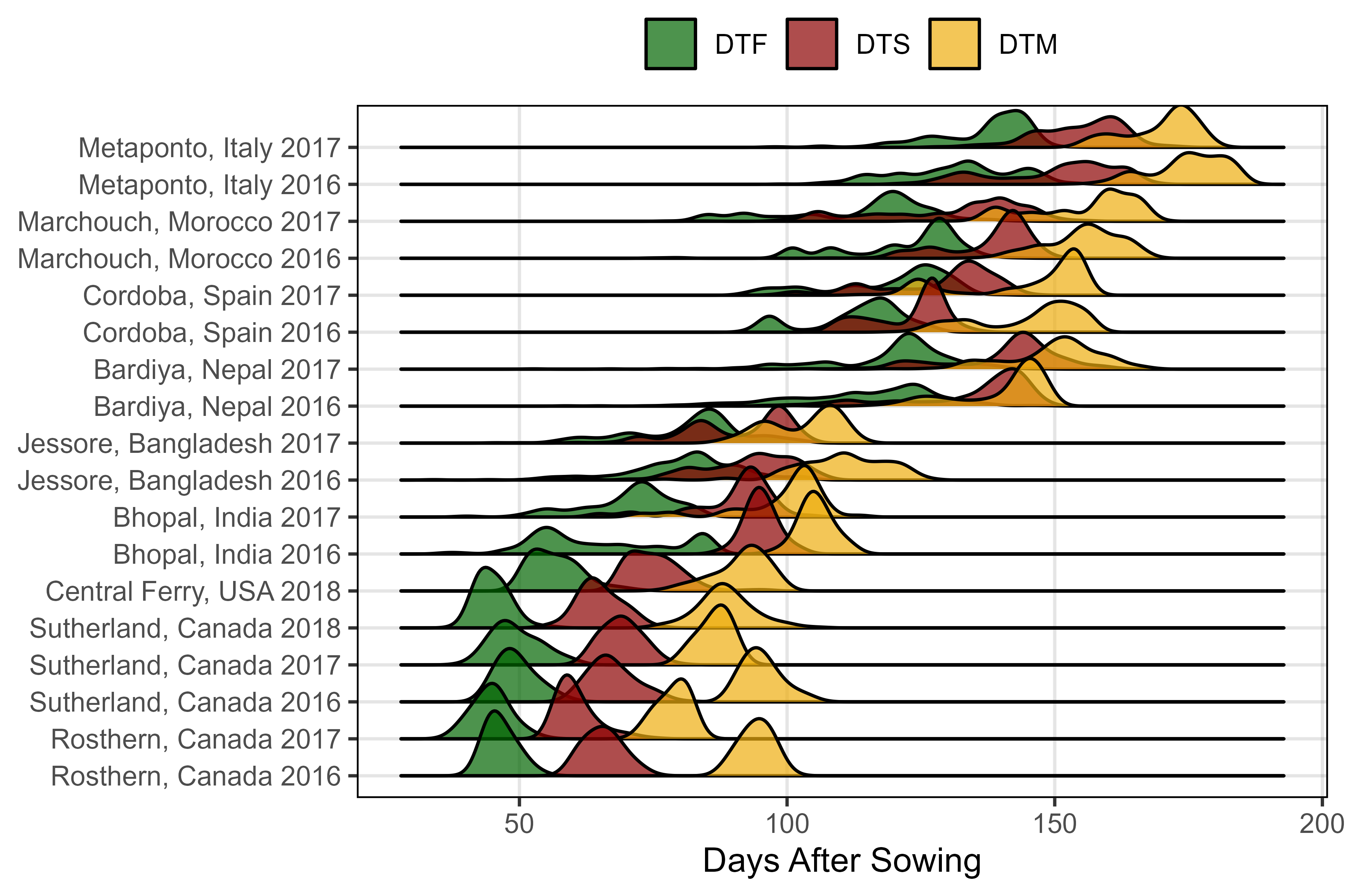
# Prep data
xx <- dd %>% select(Expt, DTF, DTS, DTM) %>%
  gather(Trait, Value, DTF, DTS, DTM) %>%
  mutate(Trait = factor(Trait, levels = c("DTF", "DTS", "DTM")))
# Plot
mp <- ggplot(xx, aes(x = Value, y = Expt, fill = Trait)) +
  ggridges::geom_density_ridges(alpha = 0.7) +
  scale_fill_manual(name = NULL, values = c("darkgreen", "darkred", "darkgoldenrod2")) +
  theme_AGL +
  theme(legend.position = "top", legend.margin = unit(c(0,0,0,0), "cm")) +
  labs(y = NULL, x = "Days After Sowing")
ggsave("Additional/Additional_Figure_03.png", mp, width = 6, height = 4, dpi = 600)
Additional Figure 4: MacroEnv Phenology
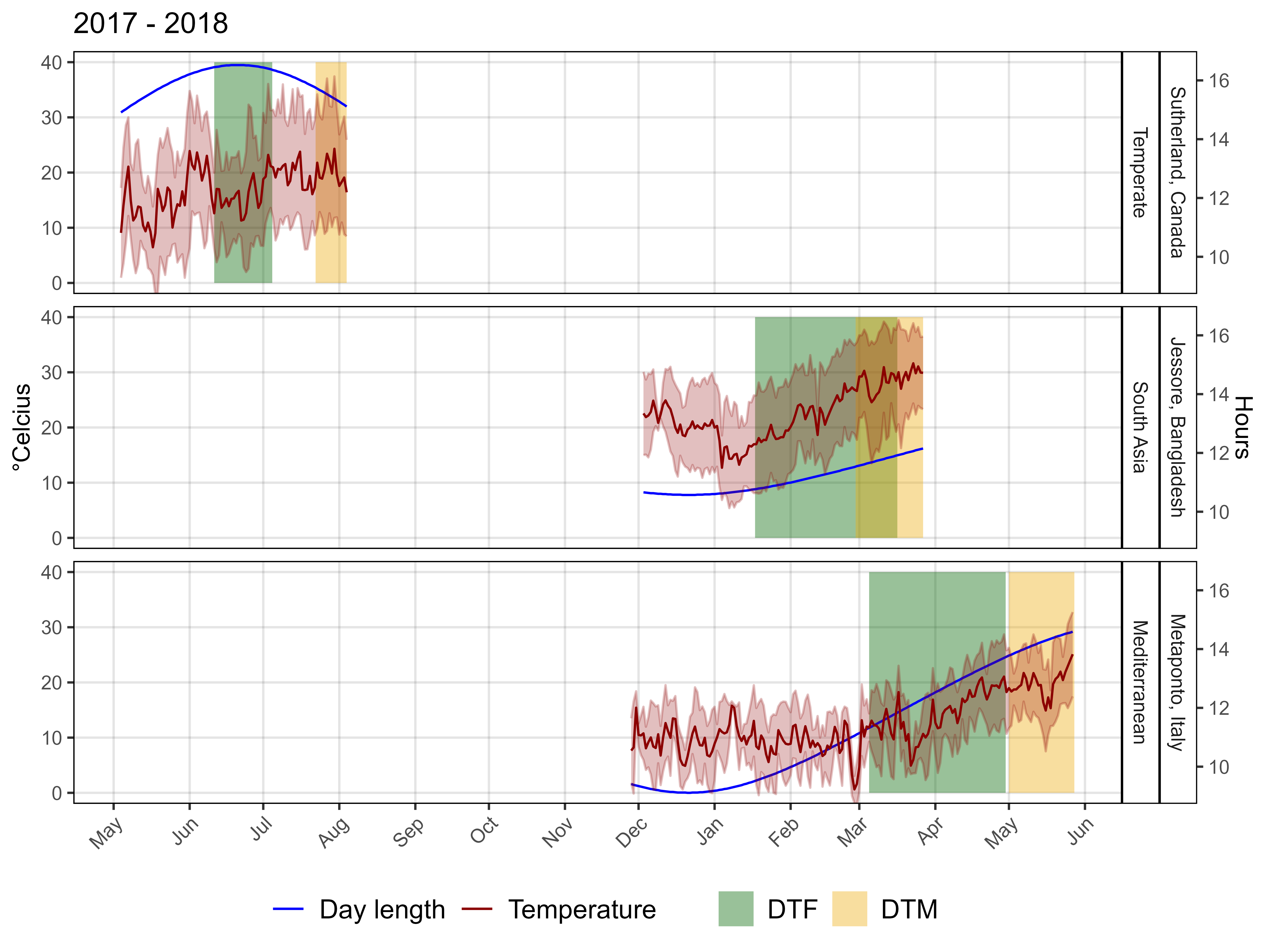
# Prep data
xx <- ee %>% filter(ExptShort %in% c("Su17", "Ba17", "It17"))
yy <- ff %>% filter(Expt %in% unique(xx$Expt)) %>%
  mutate(DTF_min = Start + DTF_min, DTF_max = Start + DTF_max,
         DTM_min = Start + DTM_min, DTM_max = Start + DTM_max)
y1 <- select(yy, Expt, Location, Year, MacroEnv, min = DTF_min, max = DTF_max) %>%
  mutate(Trait = "DTF")
y2 <- select(yy, Expt, Location, Year, MacroEnv, min = DTM_min, max = DTM_max) %>%
  mutate(Trait = "DTM")
yy <- bind_rows(y1, y2)
# Plot
mp <- ggplot(xx) +
  geom_rect(data = yy, aes(xmin = min, xmax = max, fill = Trait),
            ymin = 0, ymax = 40, alpha = 0.4) +
  geom_line(aes(x = Date, y = DayLength_rescaled, color = "Blue")) +
  geom_line(aes(x = Date, y = Temp_mean, color = "darkred") ) +
  geom_ribbon(aes(x = Date, ymin = Temp_min, ymax = Temp_max),
              fill = alpha("darkred", 0.25), color = alpha("darkred", 0.25)) +
  facet_grid(Location + MacroEnv  ~ ., scales = "free_x", space = "free_x") +
  scale_color_manual(name = NULL, values = c("Blue", "darkred"),
                    labels = c("Day length", "Temperature") ) +
  scale_fill_manual(name = NULL, values = c("darkgreen", "darkgoldenrod2")) +
  coord_cartesian(ylim = c(0,40)) +
  theme_AGL +
  theme(legend.position = "bottom",
        legend.text = element_text(size = 12),
        axis.text.x = element_text(angle = 45, hjust = 1)) +
  scale_x_date(breaks = "1 month", labels = date_format("%b")) +
  scale_y_continuous(sec.axis = sec_axis(~ (16.62 - 9.11) * . / (40 - 0) + 9.11,
                     breaks = c(10, 12, 14, 16), name = "Hours")) +
  guides(colour = guide_legend(order = 1, override.aes = list(size = 1.25)),
         fill   = guide_legend(order = 2)) +
  labs(title = "2017 - 2018", x = NULL,
       y = expression(paste(degree, "Celcius")))

ggsave("Additional/Additional_Figure_04.png", mp, width = 8, height = 6, dpi = 600)
Additional Figures: Phenology + EnvData
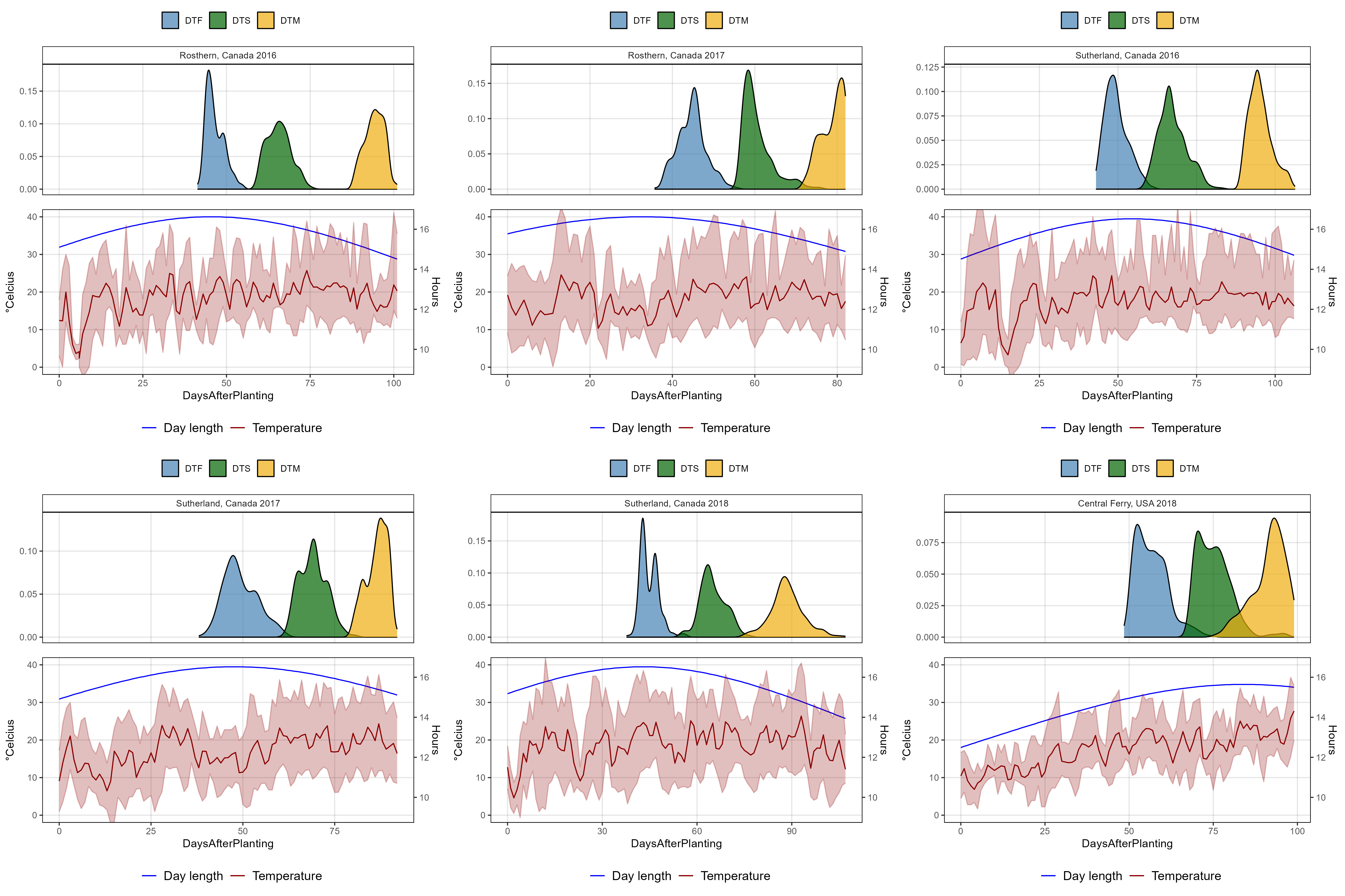
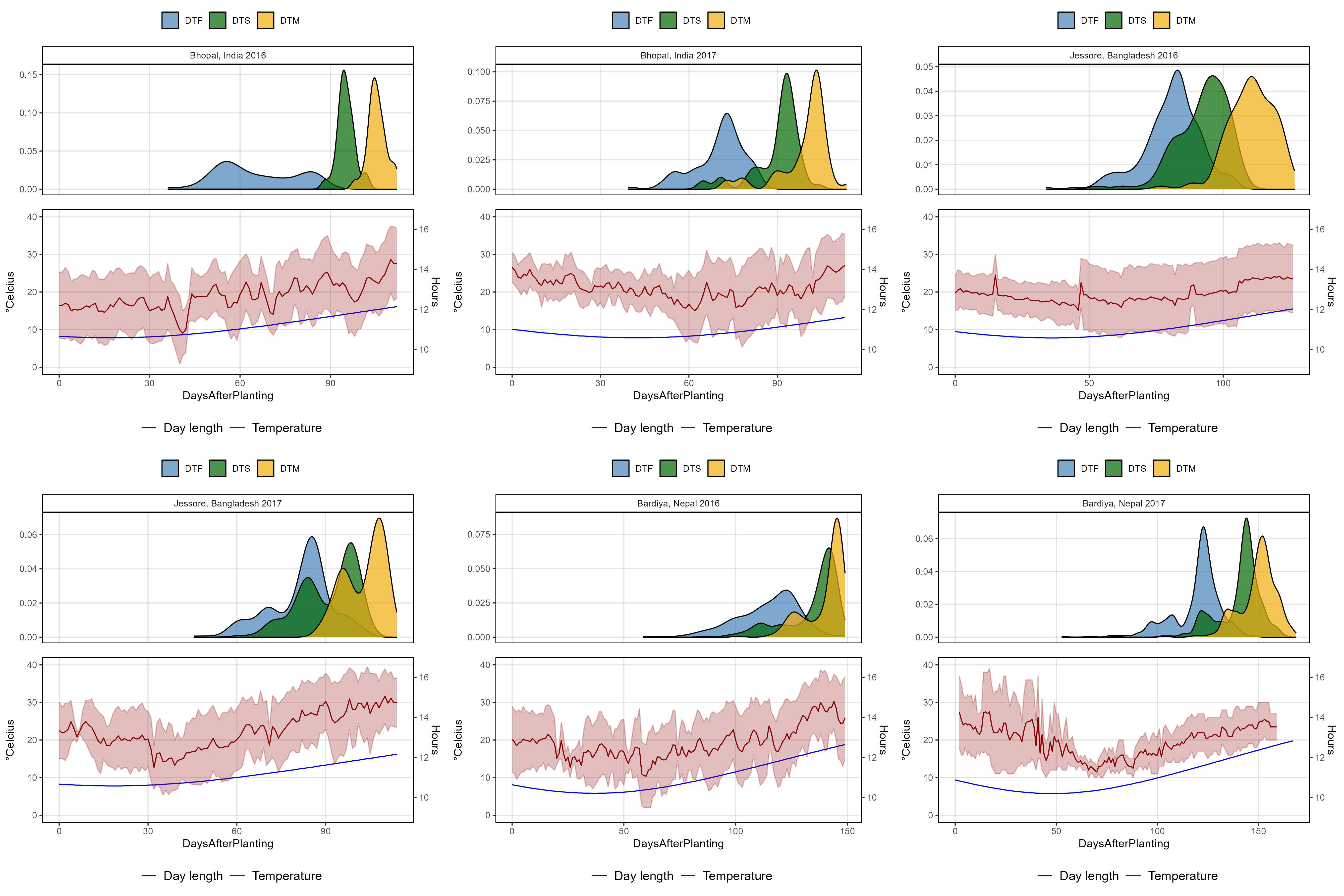
# Plotting function
ggPhenologyEnvD <- function(exptshort = "Ro17") {
  # Prep data
  x1 <- dd %>% filter(ExptShort == exptshort) %>%
    select(Entry, Name, ExptShort, Expt, DTF, DTS, DTM) %>%
    gather(Trait, Value, DTF, DTS, DTM) %>%
    mutate(Trait = factor(Trait, levels = c("DTF", "DTS", "DTM")))
  x2 <- ee %>% filter(ExptShort == exptshort)
  myMax <- max(x2$DaysAfterPlanting)
  myColors <- c("steelblue", "darkgreen", "darkgoldenrod2")
  # Plot
  mp1 <- ggplot(x1, aes(x = Value, fill = Trait)) +
    geom_density(alpha = 0.7) +
    facet_grid(. ~ Expt) +
    scale_fill_manual(name = NULL, values = myColors) +
    coord_cartesian(xlim = c(0,myMax)) +
    theme_AGL +
    theme(legend.position = "top",
          axis.text.x  = element_blank(),
          axis.ticks.x = element_blank()) +
    labs(x = NULL, y = NULL)
  mp2 <- ggplot(x2) +
    geom_line(aes(x = DaysAfterPlanting, y = DayLength_rescaled, color = "Blue")) +
    geom_line(aes(x = DaysAfterPlanting, y = Temp_mean, color = "darkred") ) +
    geom_ribbon(aes(x = DaysAfterPlanting, ymin = Temp_min, ymax = Temp_max),
                fill = alpha("darkred", 0.25), color = alpha("darkred", 0.25)) +
    scale_color_manual(name = NULL, values = c("Blue", "darkred"),
                       labels = c("Day length", "Temperature") ) +
    coord_cartesian(ylim = c(0,40)) +
    theme_AGL +
    theme(legend.position = "bottom",
          legend.text = element_text(size = 12)) +
    scale_x_continuous(limits = c(0, myMax)) +
    scale_y_continuous(sec.axis = sec_axis(~ (16.62 - 9.11) * . / (40 - 0) + 9.11,
                          breaks = c(10, 12, 14, 16), name = "Hours")) +
    guides(colour = guide_legend(order = 1, override.aes = list(size = 1.25)),
           fill   = guide_legend(order = 2)) +
    labs(y = expression(paste(degree, "Celcius"), x = NULL))
  ggarrange(mp1, mp2, nrow = 2, align = "v", heights = c(1, 1.2))
}
for(i in names_ExptShort) {
  mp <- ggPhenologyEnvD(i)
  ggsave(paste0("Additional/Expt/1_", i, ".png"), width = 6, height = 6)
}
im <- image_read(paste0("Additional/Expt/1_", names_ExptShort[1:6], ".png"))
im <- image_append(c(image_append(im[1:3]), image_append(im[4:6])), stack = T)
image_write(im, "Additional/Expt/2_Temperate.png")
im <- image_read(paste0("Additional/Expt/1_", names_ExptShort[7:12], ".png"))
im <- image_append(c(image_append(im[1:3]), image_append(im[4:6])), stack = T)
image_write(im, "Additional/Expt/2_SouthAsia.png")
im <- image_read(paste0("Additional/Expt/1_", names_ExptShort[13:18], ".png"))
im <- image_append(c(image_append(im[1:3]), image_append(im[4:6])), stack = T)
image_write(im, "Additional/Expt/2_Mediterranean.png")
Supplemental Figure 2: Missing Data
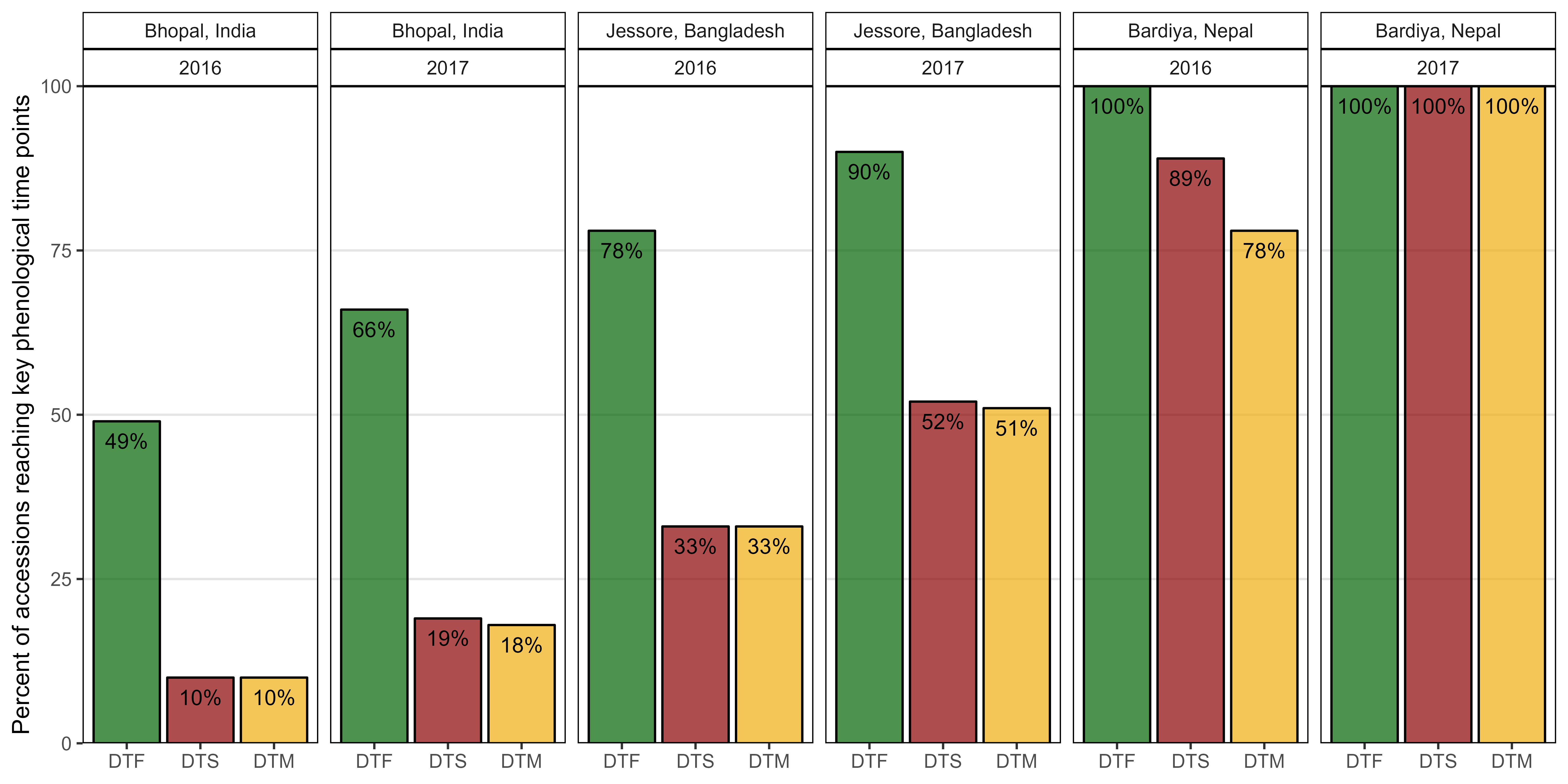
Figure S2: Percentage of lentil genotypes reaching key phenological time points in South Asian locations. Days from sowing to: flowering (DTF), swollen pods (DTS) and maturity (DTM).
# Prep data
xx <- dd %>%
  filter(Location %in% c("Bhopal, India", "Jessore, Bangladesh", "Bardiya, Nepal")) %>%
  mutate(DTF = ifelse(is.na(DTF), 0, 1),
         DTS = ifelse(is.na(DTS), 0, 1),
         DTM = ifelse(is.na(DTM), 0, 1) ) %>%
  group_by(Expt, Location, Year) %>%
  summarise_at(vars(DTF, DTS, DTM), funs(sum), na.rm = T) %>%
  ungroup() %>%
  gather(Trait, Flowered, DTF, DTS, DTM) %>%
  mutate(Total = ifelse(Expt == "Bardiya, Nepal 2016", 323, 324),
         # One accession was not planted in Bardiya, Nepal 2016
         DidNotFlower = Total - Flowered,
         Percent = round(100 * Flowered / Total),
         Label = paste0(Percent, "%"),
         Trait = factor(Trait, levels = c("DTF", "DTS", "DTM")))
# Plot
mp <- ggplot(xx, aes(x = Trait, y = Percent, fill = Trait)) +
  geom_bar(stat = "identity", color = "black", alpha = 0.7) +
  geom_text(aes(label = Label), nudge_y = -3, size = 3.5) +
  facet_grid(. ~ Location + Year) +
  scale_fill_manual(values = c("darkgreen", "darkred", "darkgoldenrod2")) +
  scale_y_continuous(limits = c(0,100), expand = c(0,0)) +
  theme_AGL +
  theme(legend.position = "none",
        panel.grid.major.x = element_blank() ) +
  labs(x = NULL, y = "Percent of accessions reaching key phenological time points")
ggsave("Supplemental_Figure_02.png", width = 10, height = 5, dpi = 600)
Supplemental Figure 3: Correlation Plots
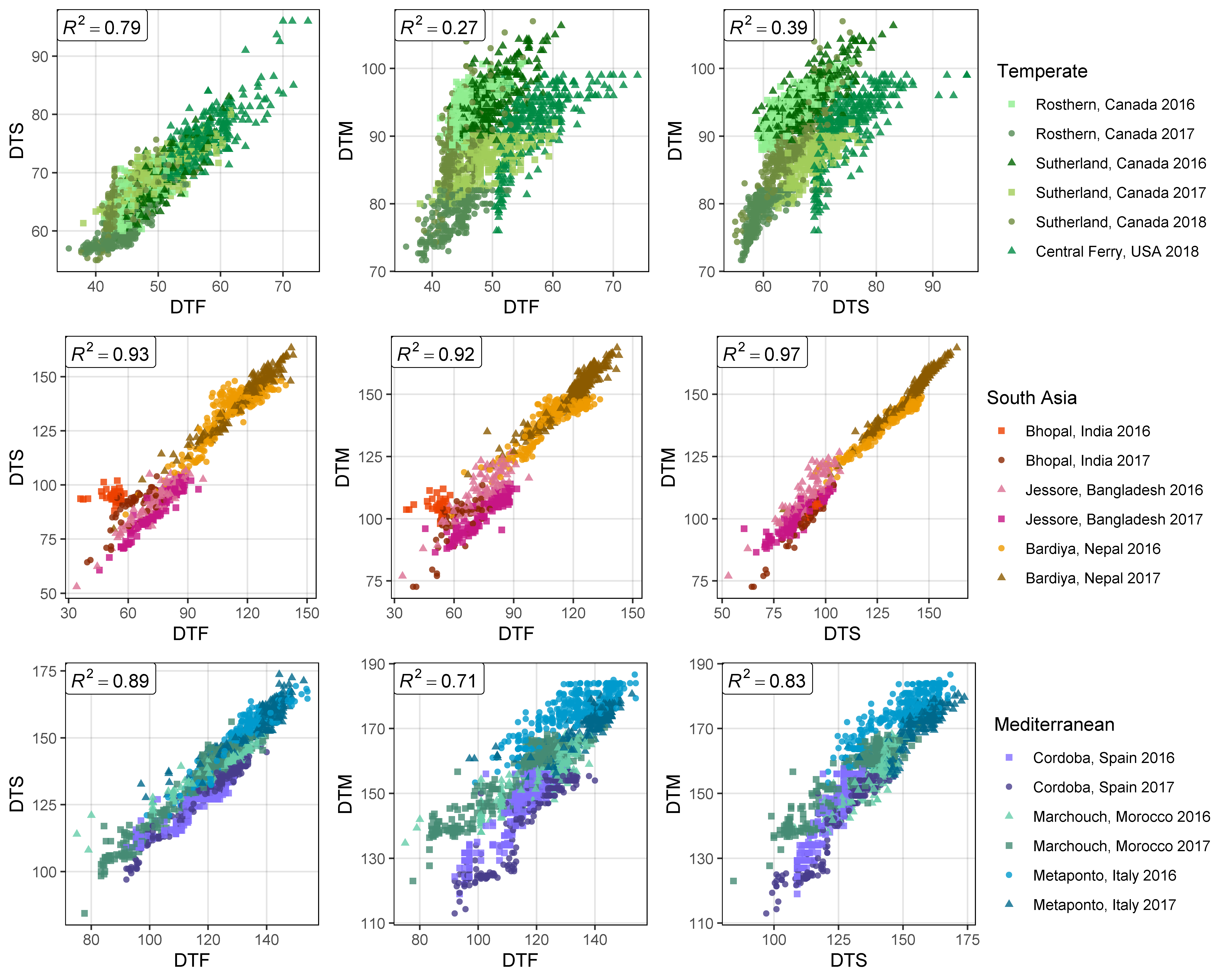
Figure S3: Correlations along with the corresponding correlation coefficients (R2) between days from sowing to: flowering (DTF), swollen pod (DTS) and maturity (DTM), in temperate (top), South Asian (middle) and Mediterranean (bottom) locations.
# Prep data
xx <- dd %>%
  left_join(select(ff, Expt, MacroEnv), by = "Expt") %>%
  select(Entry, Expt, MacroEnv, DTF, DTS, DTM)
# Create plotting function
ggCorPlot <- function(x, legend.title, colNums) {
  # Plot (a)
  r2 <- round(cor(x$DTF, x$DTS, use ="complete", method = "pearson")^2, 2)
  tp1 <- ggplot(x) +
    geom_point(aes(x = DTF, y = DTS, color = Expt, shape = Expt), alpha = 0.8) +
    geom_label(x = -Inf, y = Inf, hjust = 0, vjust = 1, parse = T,
               label = paste("italic(R)^2 == ", r2) ) +
    scale_color_manual(name = legend.title, values = colors_Expt[colNums]) +
    scale_shape_manual(name = legend.title, values = c(15,16,17,15,16,17)) +
    theme_AGL
  # Plot (b)
  r2 <- round(cor(x$DTF, x$DTM, use ="complete.obs", method = "pearson")^2, 2)
  tp2 <- ggplot(x) +
    geom_point(aes(x = DTF, y = DTM, color = Expt, shape = Expt), alpha = 0.8) +
    geom_label(x = -Inf, y = Inf, hjust = 0, vjust = 1, parse = T,
               label = paste("italic(R)^2 == ", r2) ) +
    scale_color_manual(name = legend.title, values = colors_Expt[colNums]) +
    scale_shape_manual(name = legend.title, values = c(15,16,17,15,16,17)) +
    theme_AGL
  # Plot (c)
  r2 <- round(cor(x$DTS, x$DTM, use = "complete", method = "pearson")^2, 2)
  tp3 <- ggplot(x) +
    geom_point(aes(x = DTS, y = DTM, color = Expt, shape = Expt), alpha = 0.8) +
    geom_label(x = -Inf, y = Inf, hjust = 0, vjust = 1, parse = T,
               label = paste("italic(R)^2 == ", r2) ) +
    scale_color_manual(name = legend.title, values = colors_Expt[colNums]) +
    scale_shape_manual(name = legend.title, values = c(15,16,17,15,16,17)) +
    theme_AGL
  # Append (a), (b) and (c)
  mp <- ggarrange(tp1, tp2, tp3, nrow = 1, ncol = 3, common.legend = T, legend = "right")
  mp
}
# Plot
mp1 <- ggCorPlot(xx %>% filter(MacroEnv == "Temperate"),     "Temperate",      1:6 )
mp2 <- ggCorPlot(xx %>% filter(MacroEnv == "South Asia"),    "South Asia",     7:12)
mp3 <- ggCorPlot(xx %>% filter(MacroEnv == "Mediterranean"), "Mediterranean", 13:18)
mp <- ggarrange(mp1, mp2, mp3, nrow = 3, ncol = 1, common.legend = T, legend = "right")
ggsave("Supplemental_Figure_03.png", mp, width = 10, height = 8, dpi = 600)
Additional Figures: Correlations
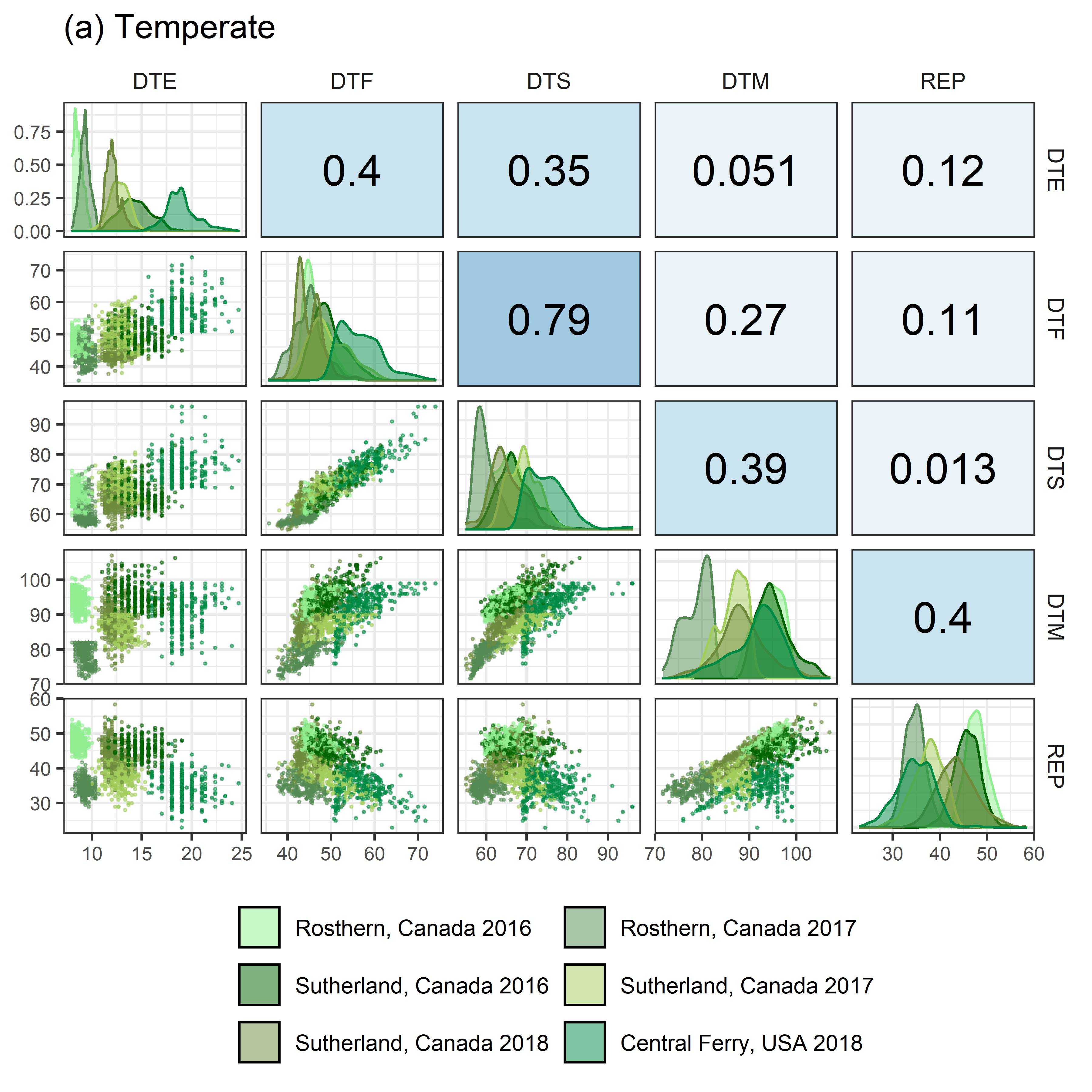
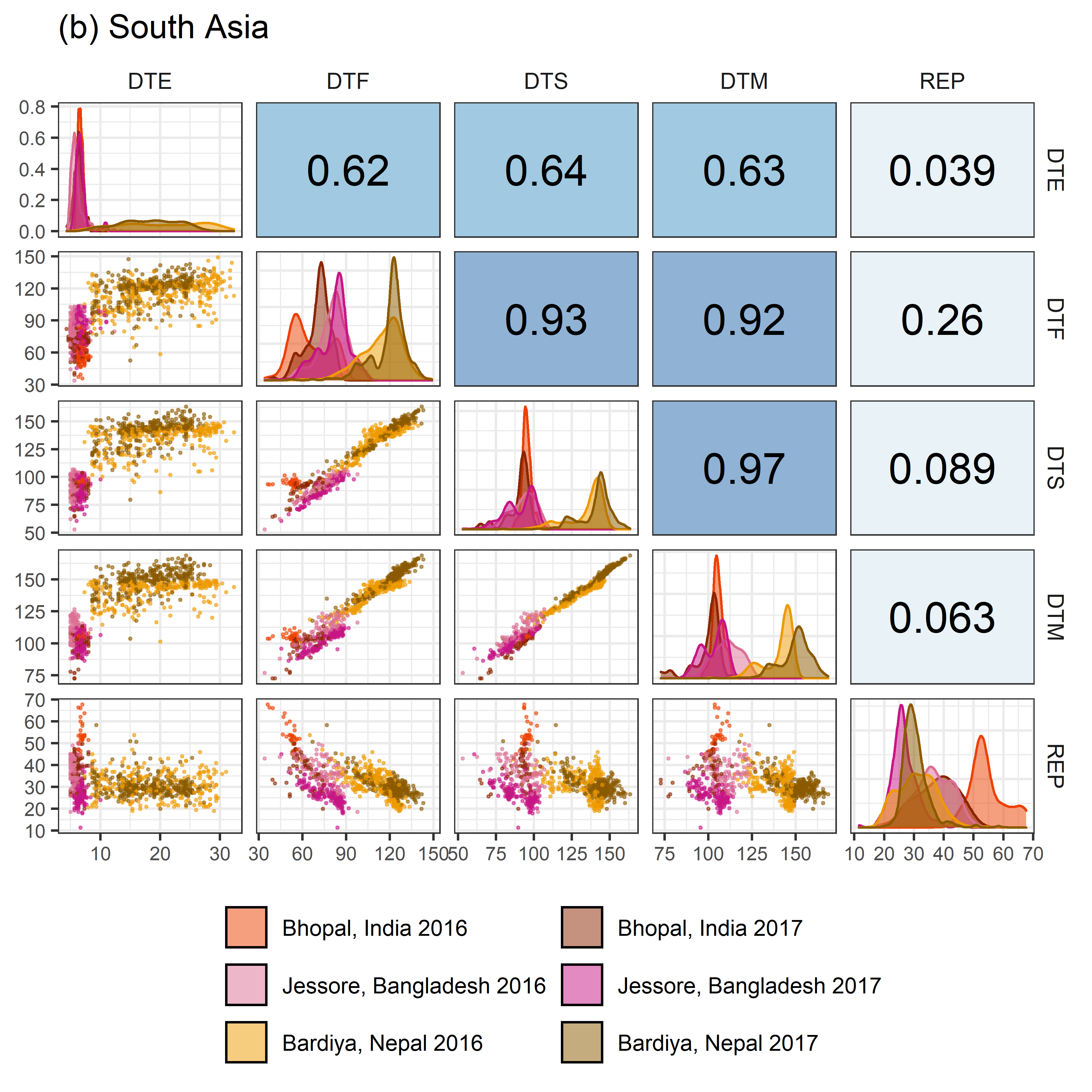
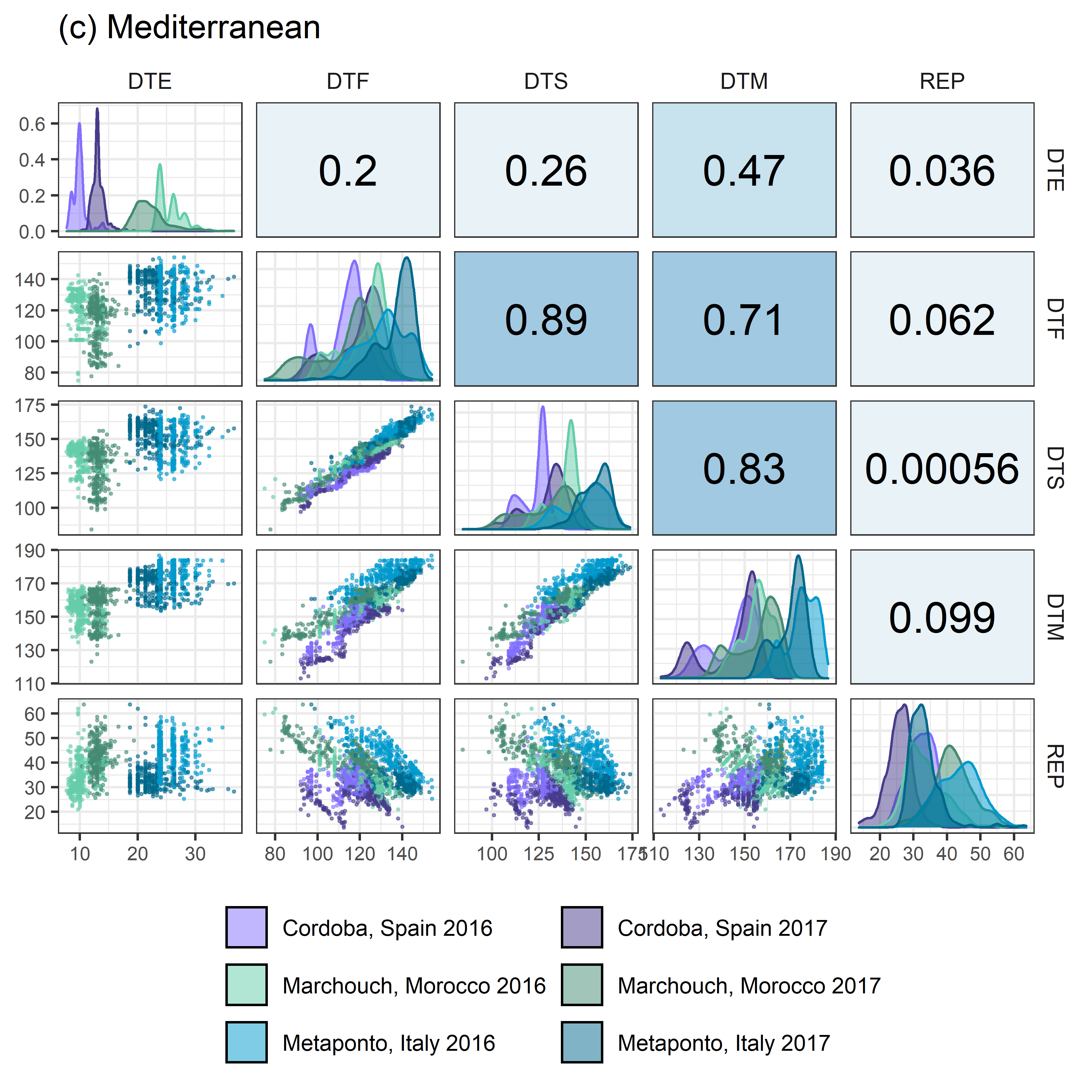
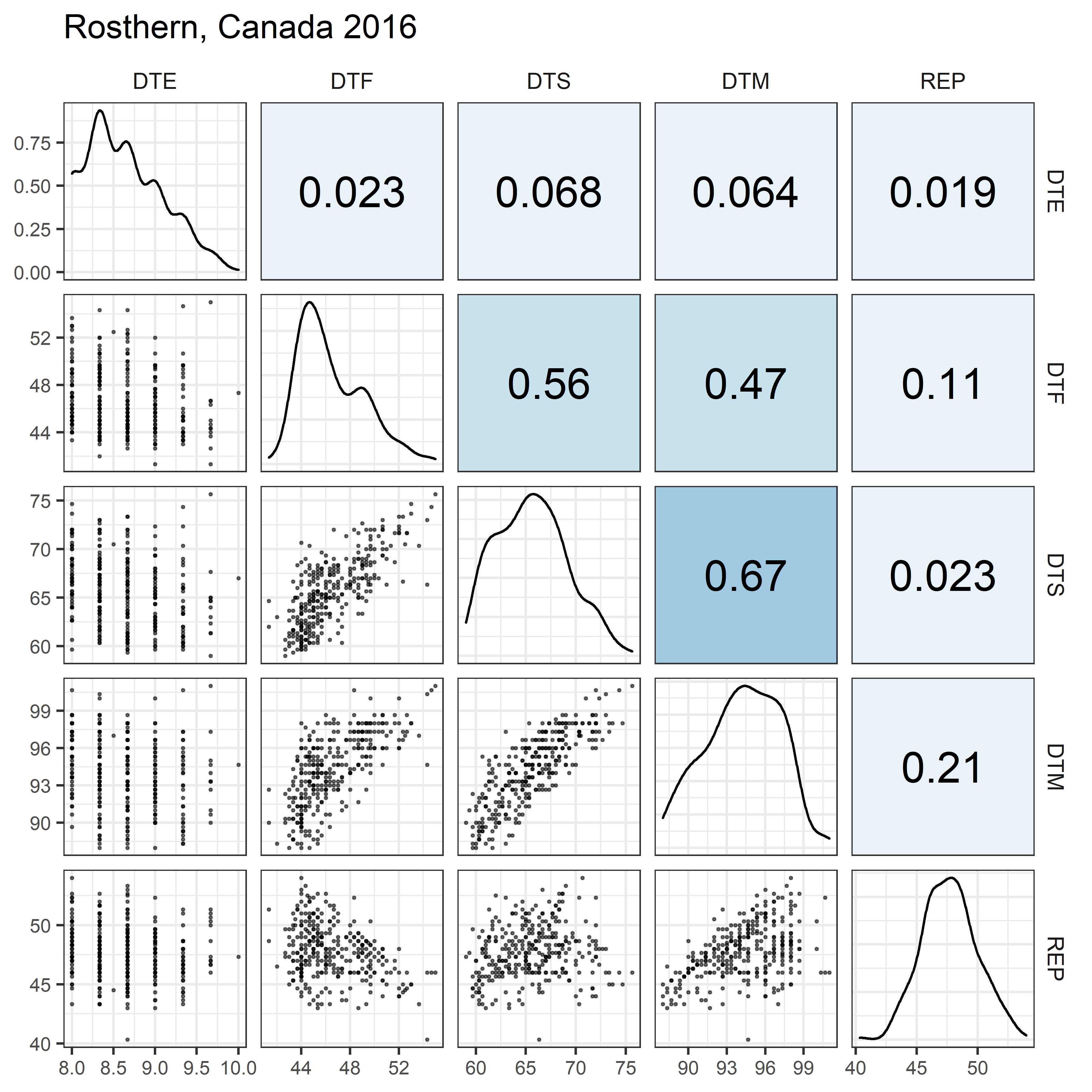
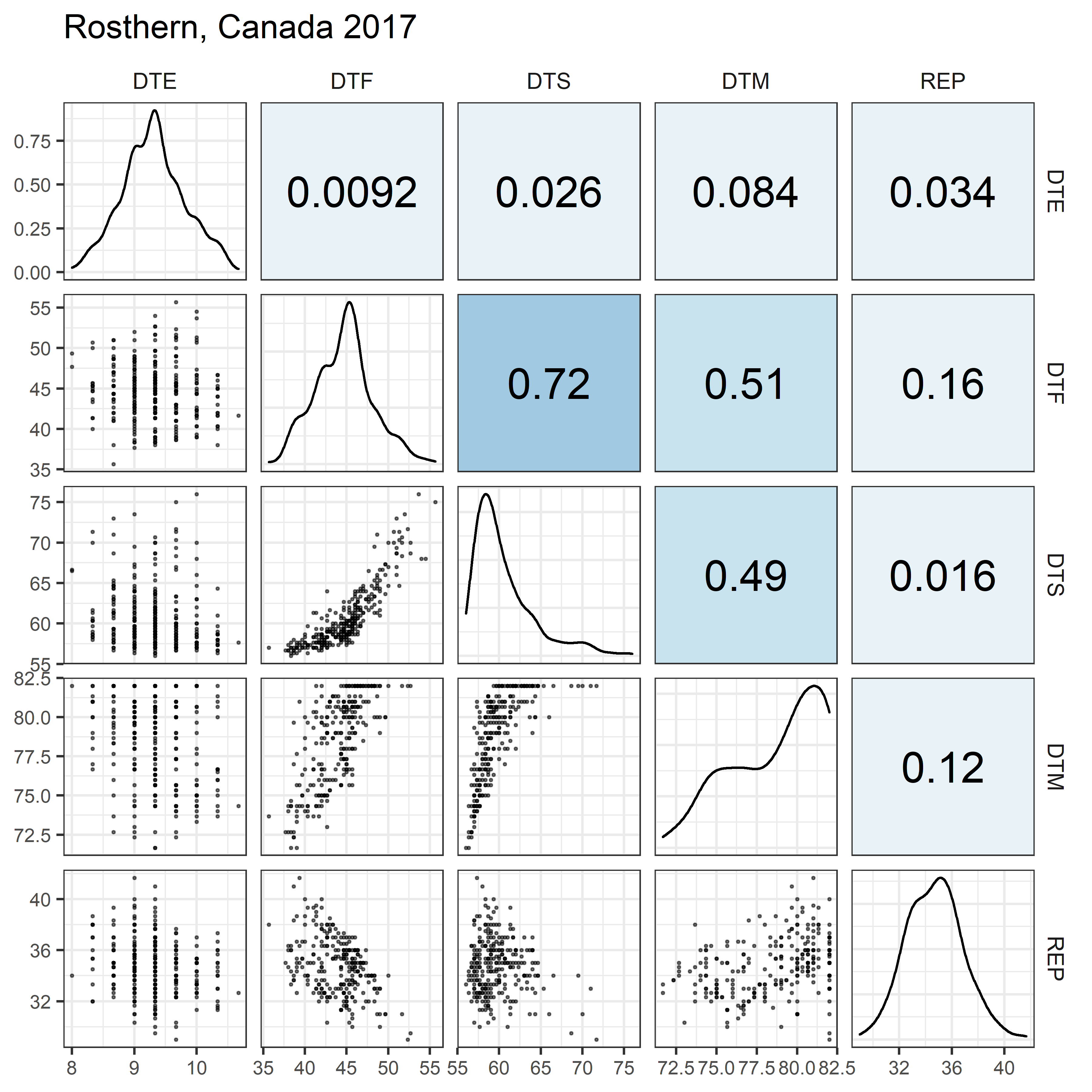
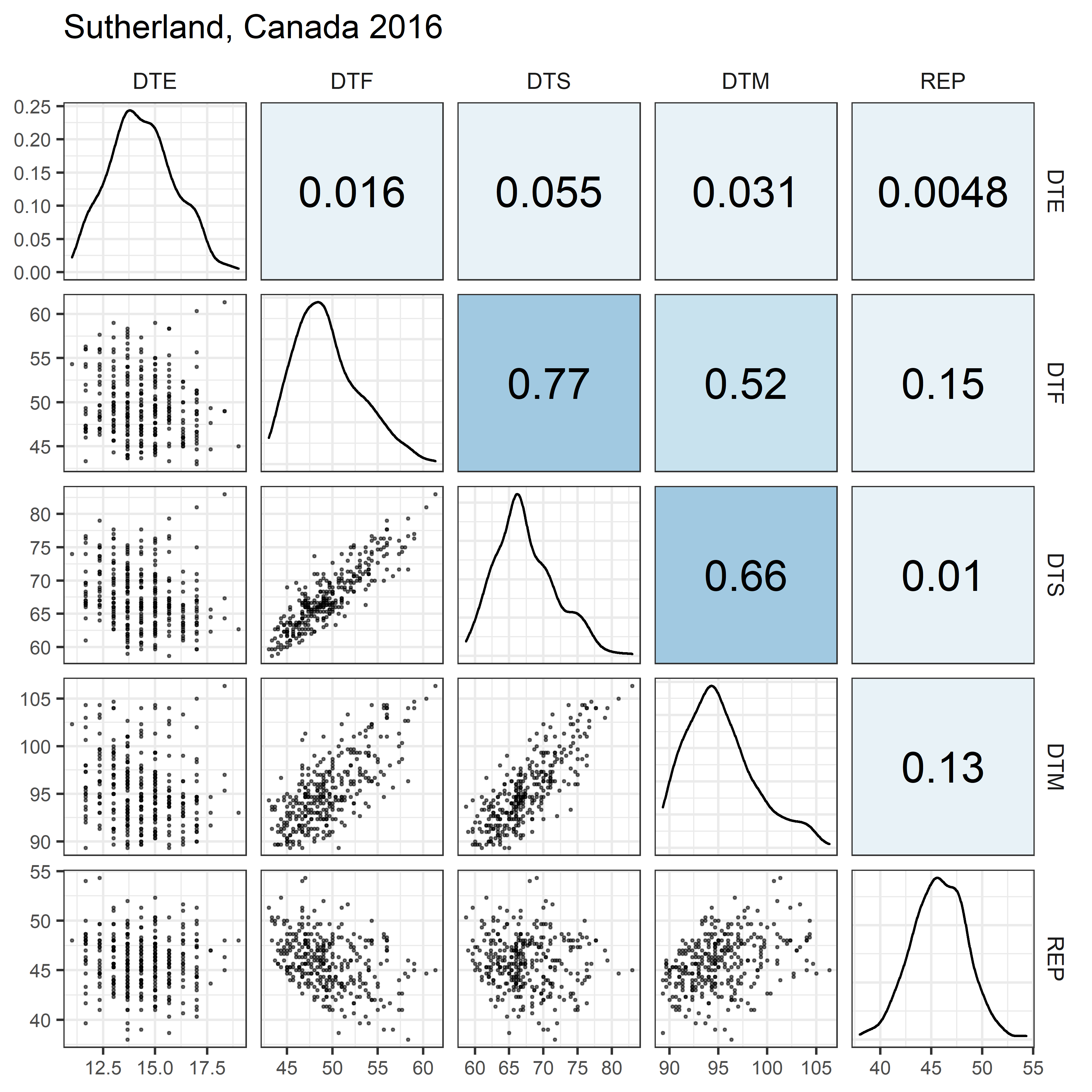
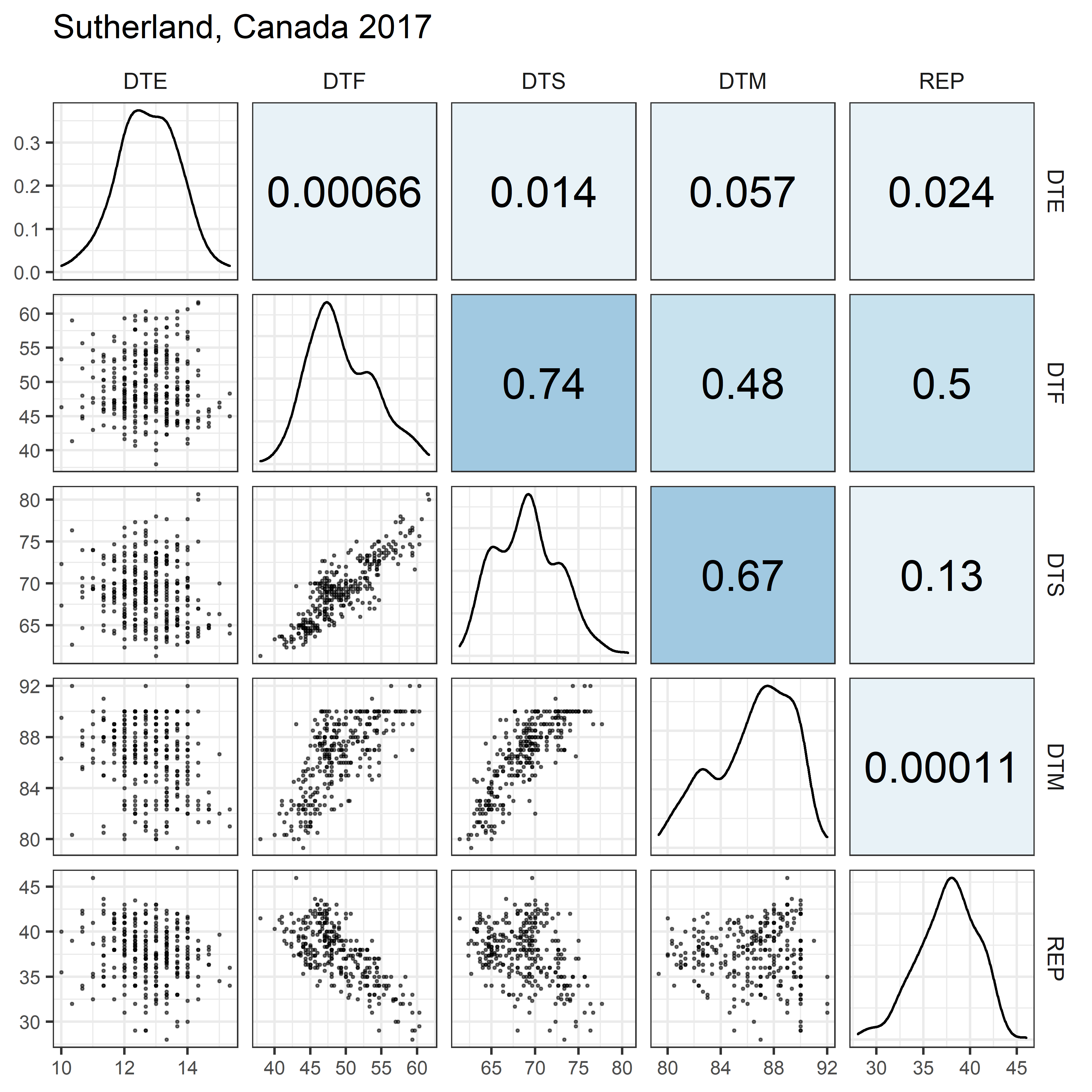
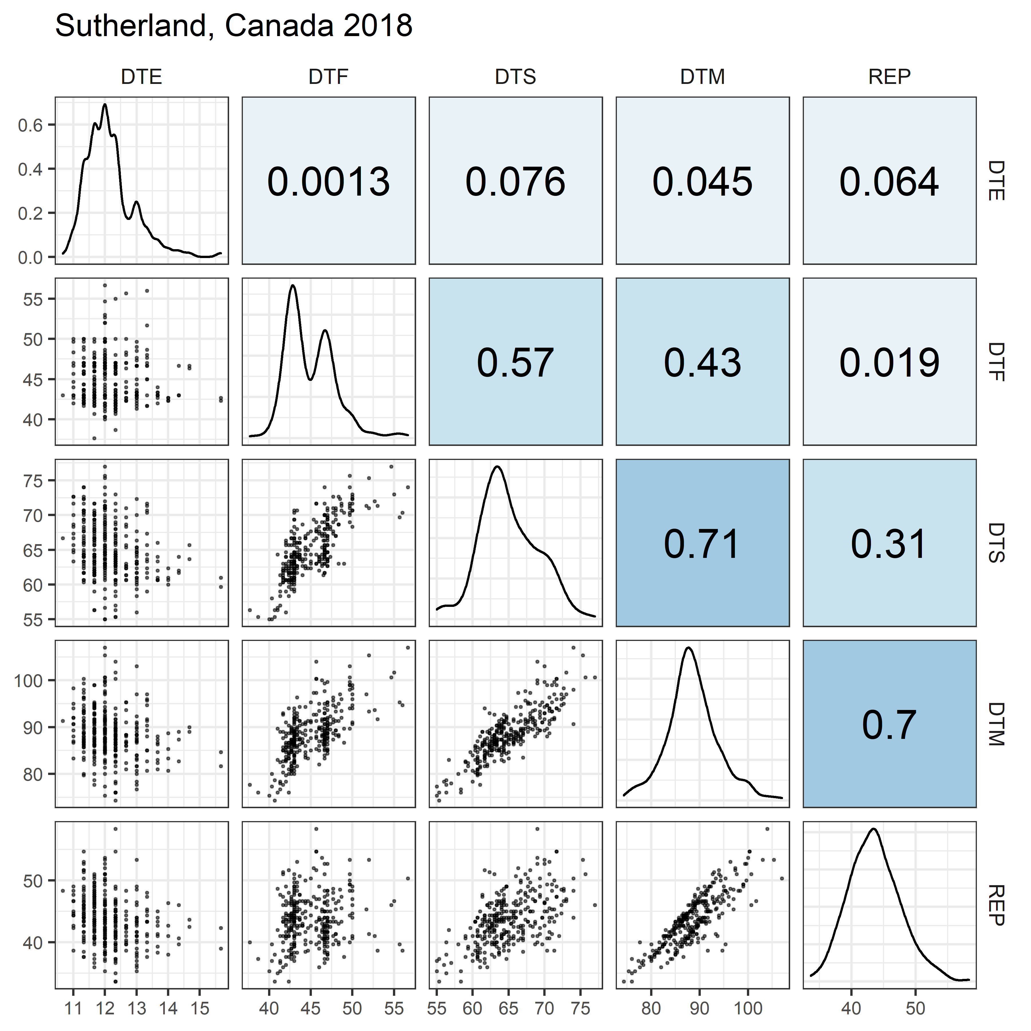
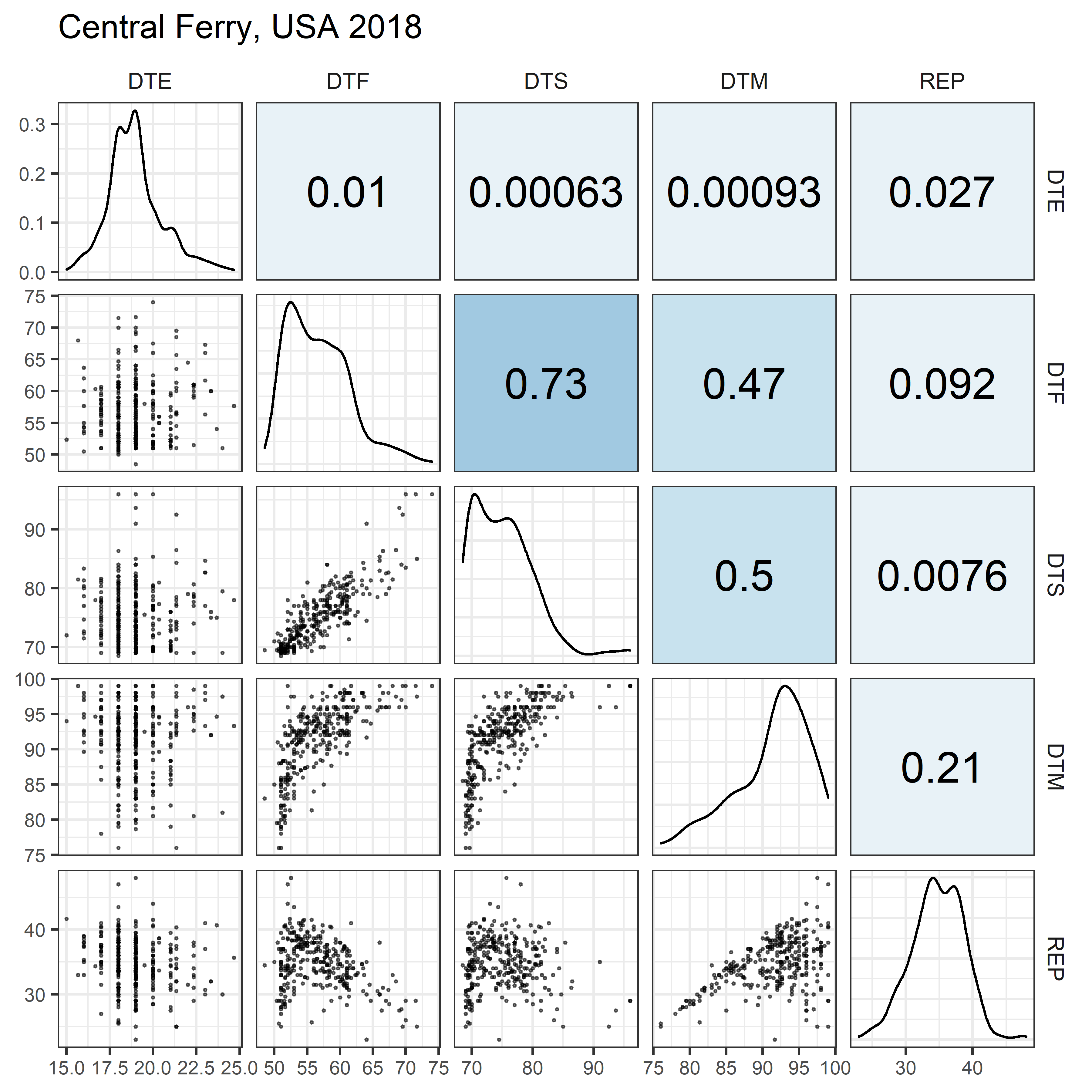

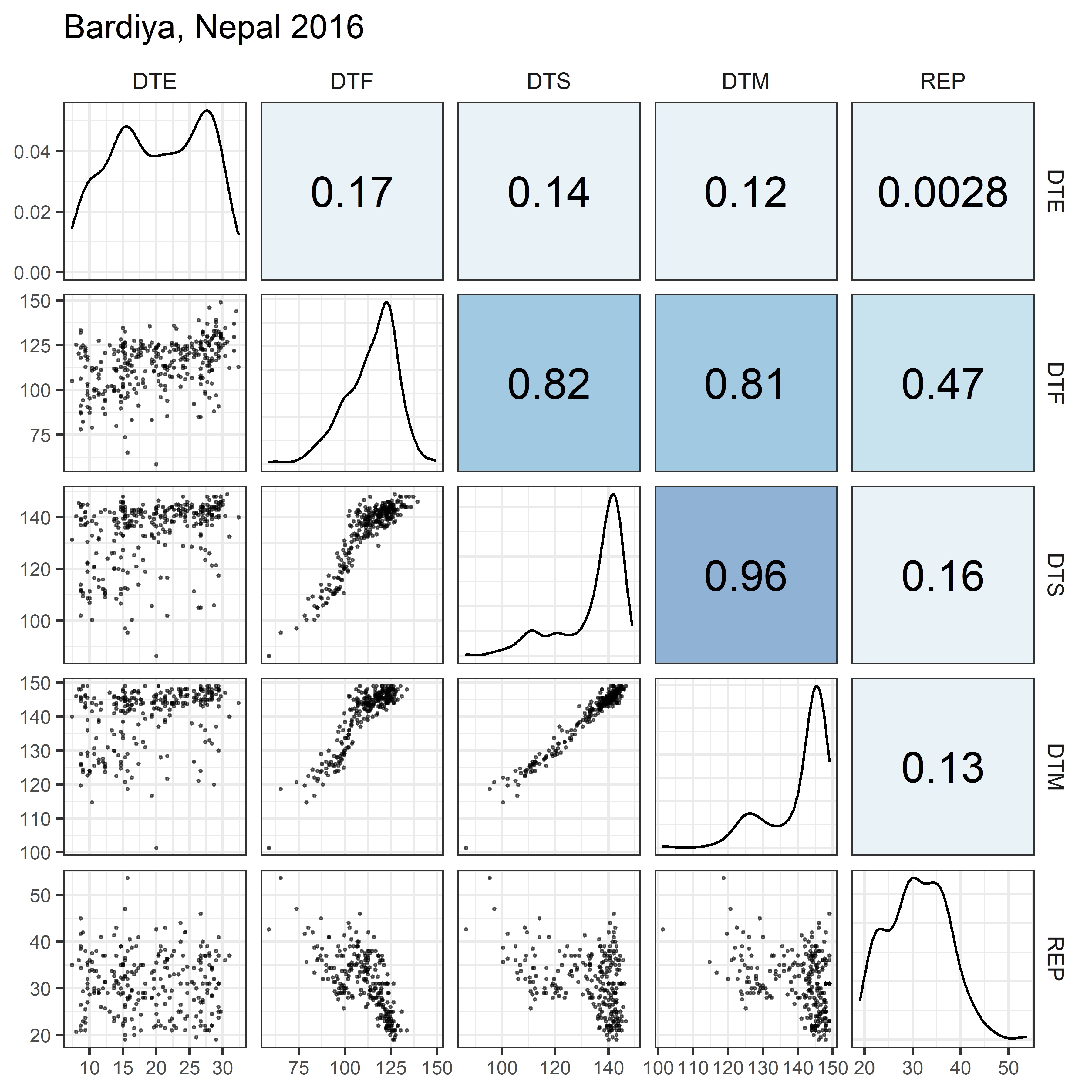
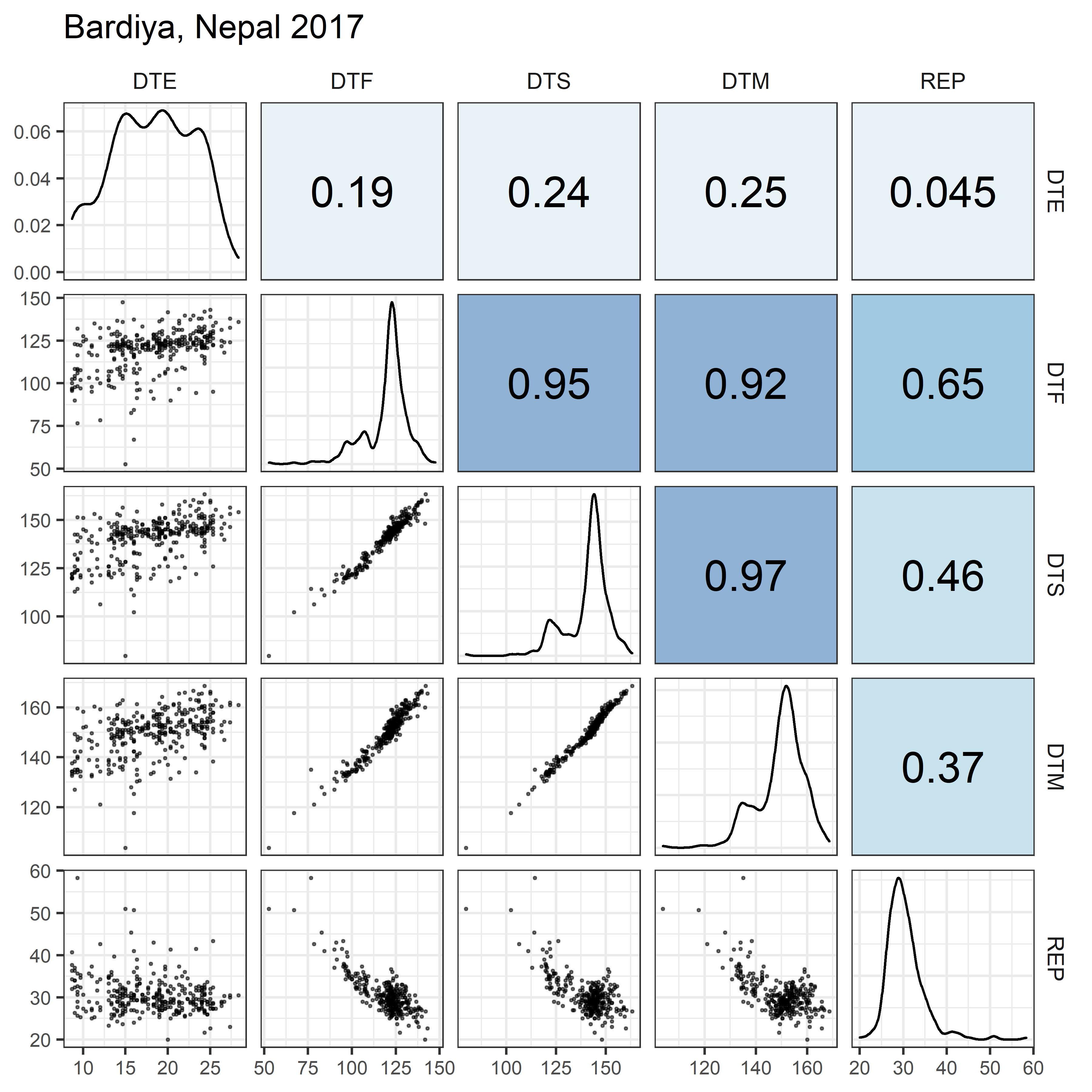
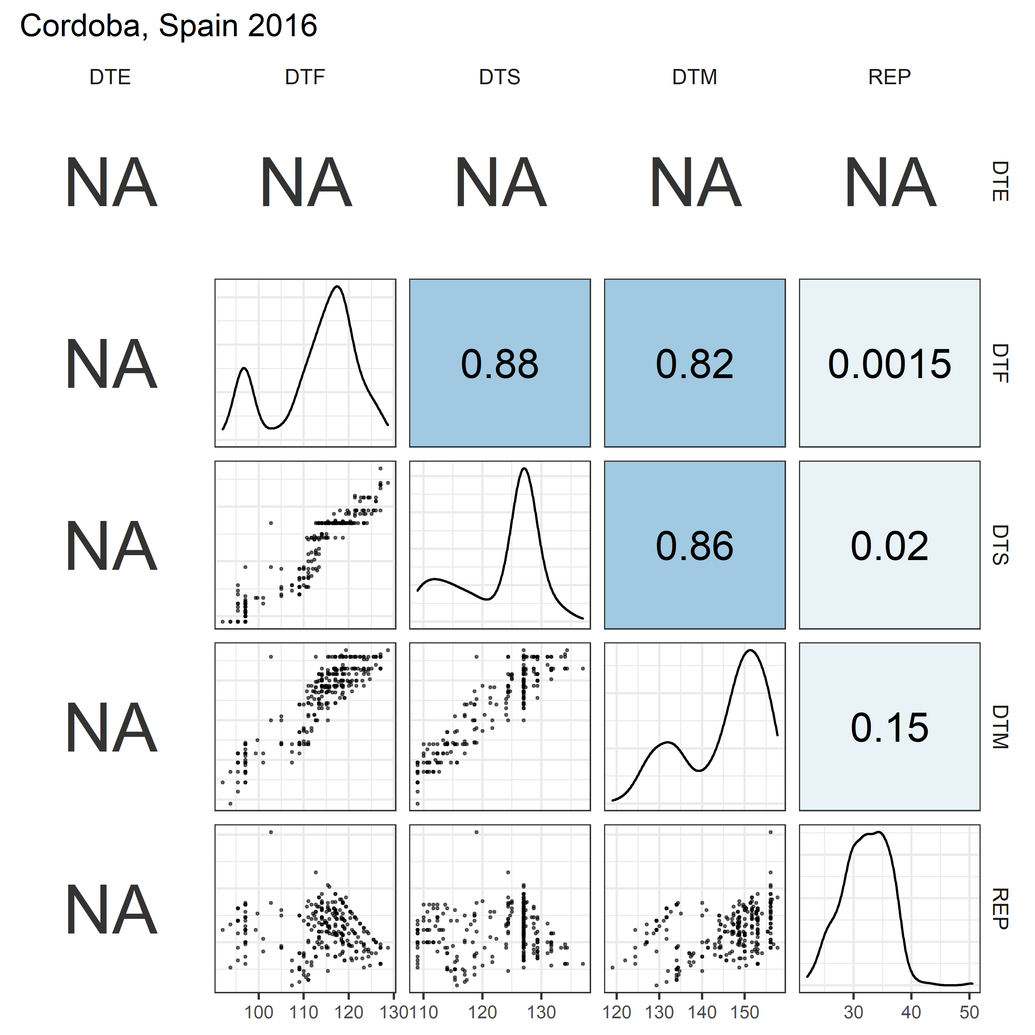
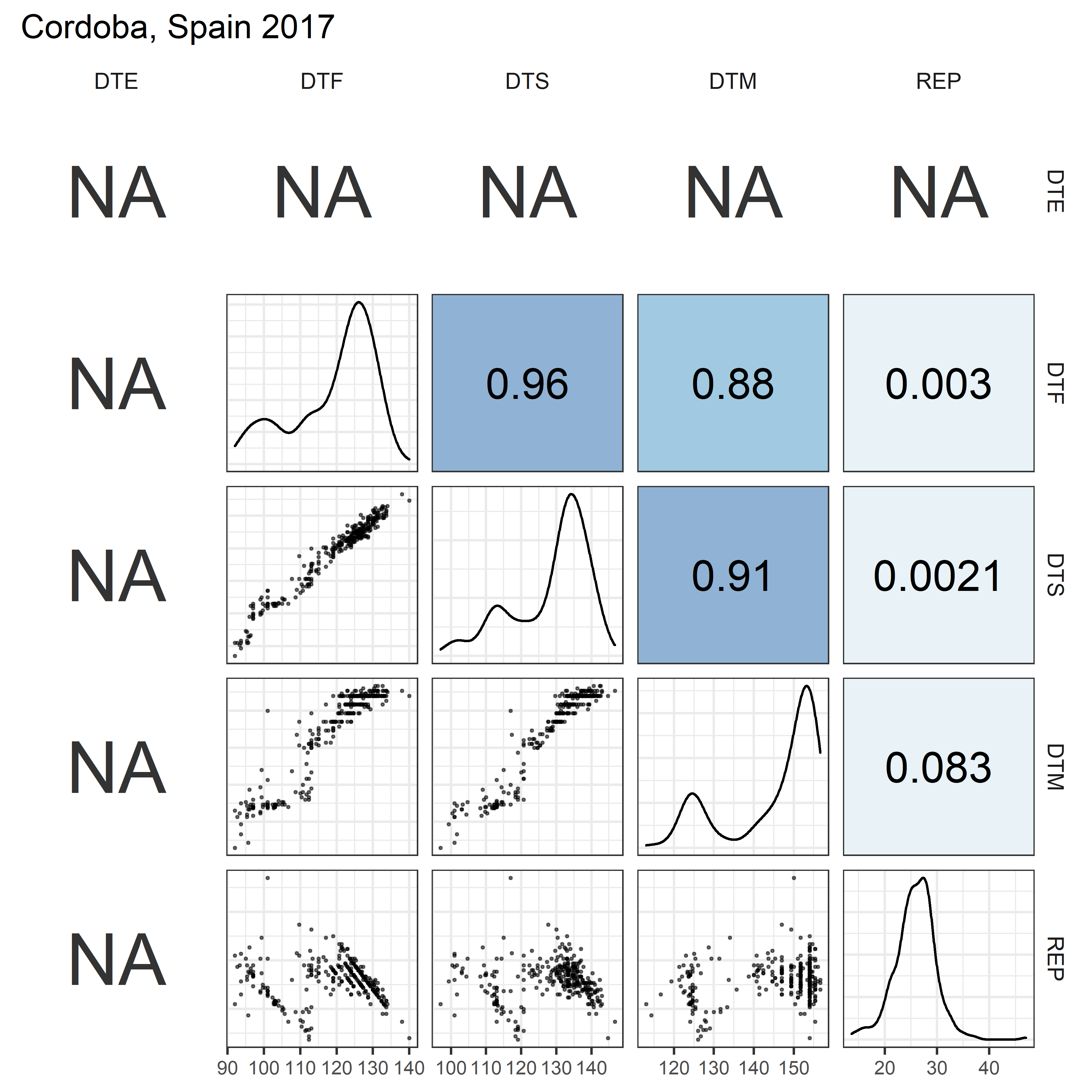
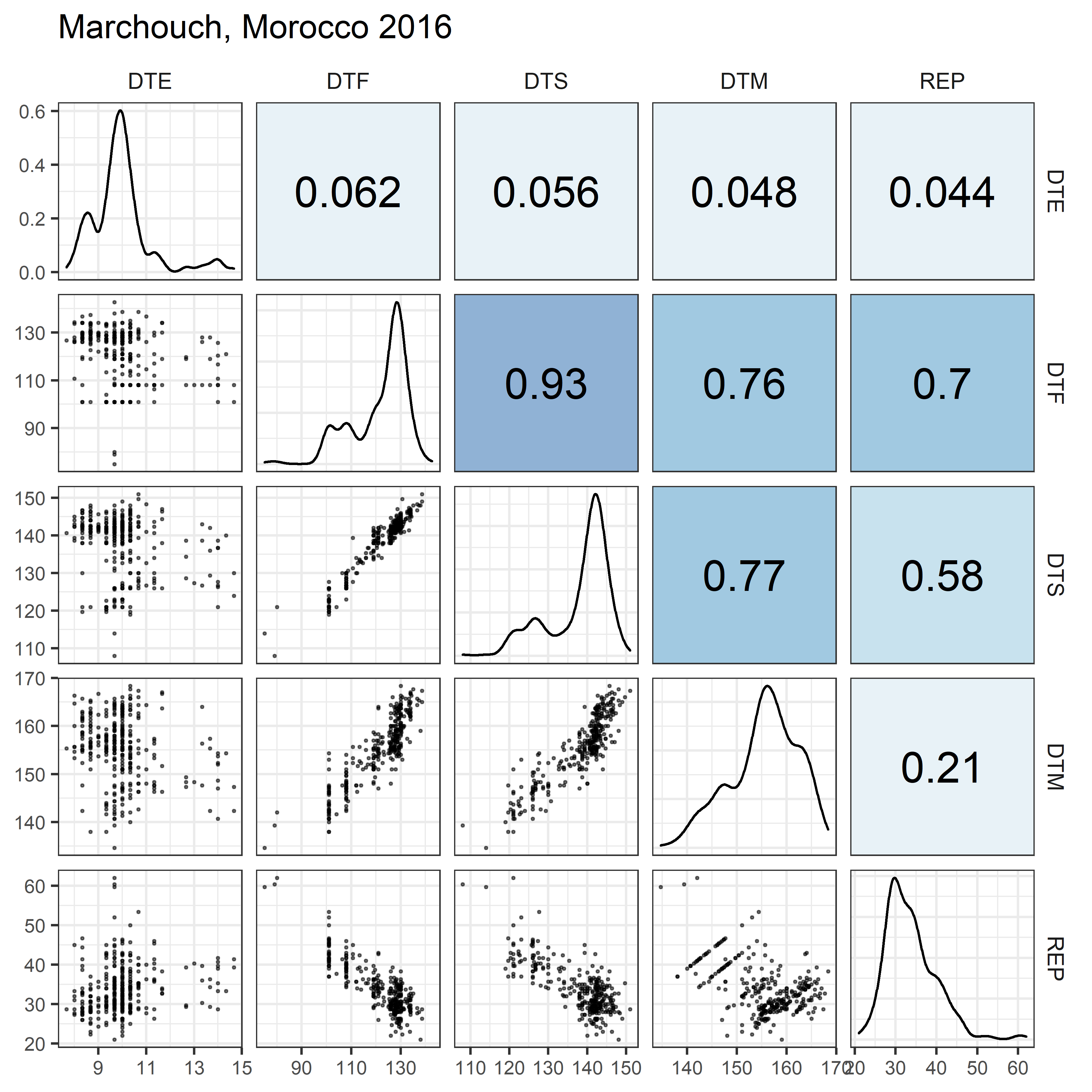
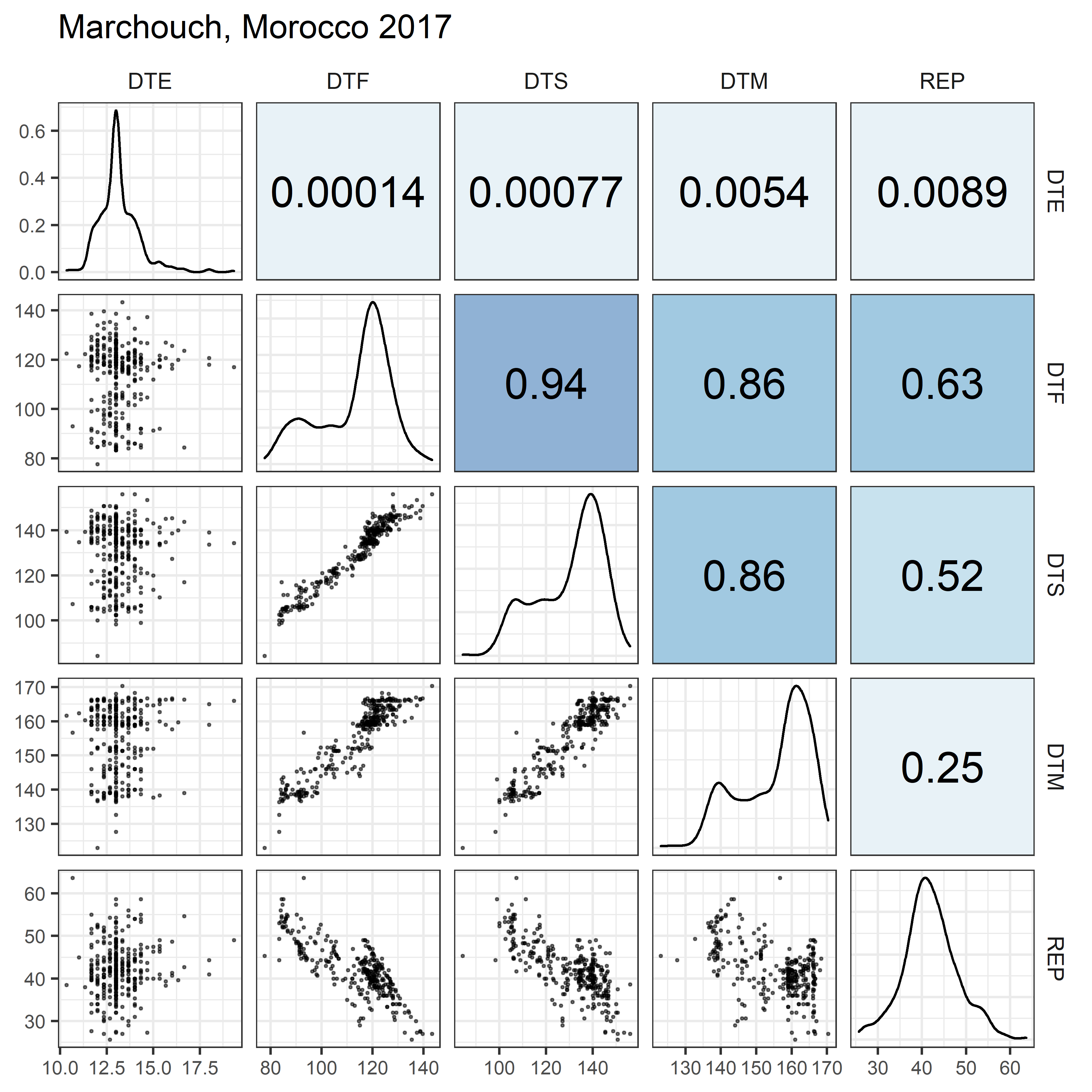
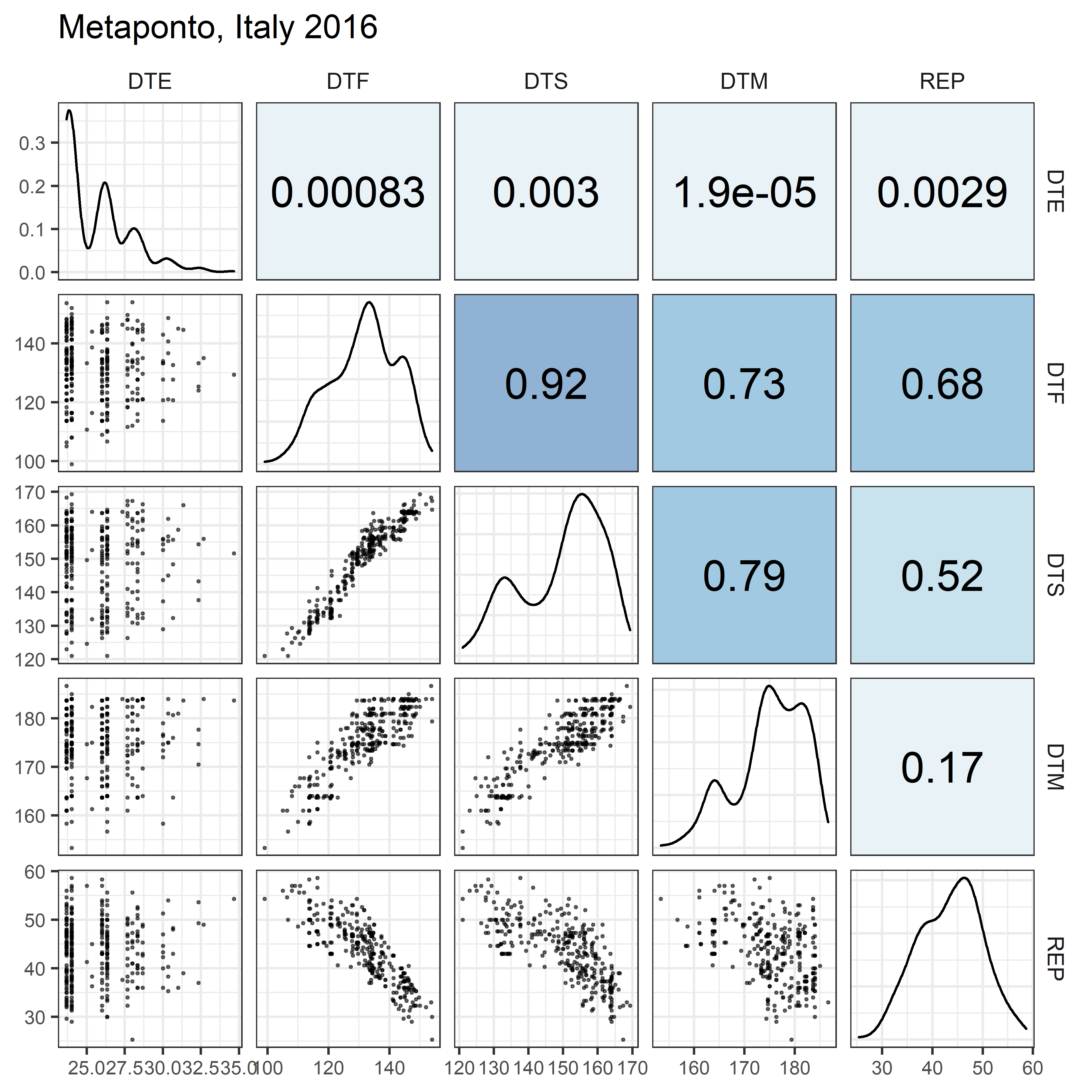
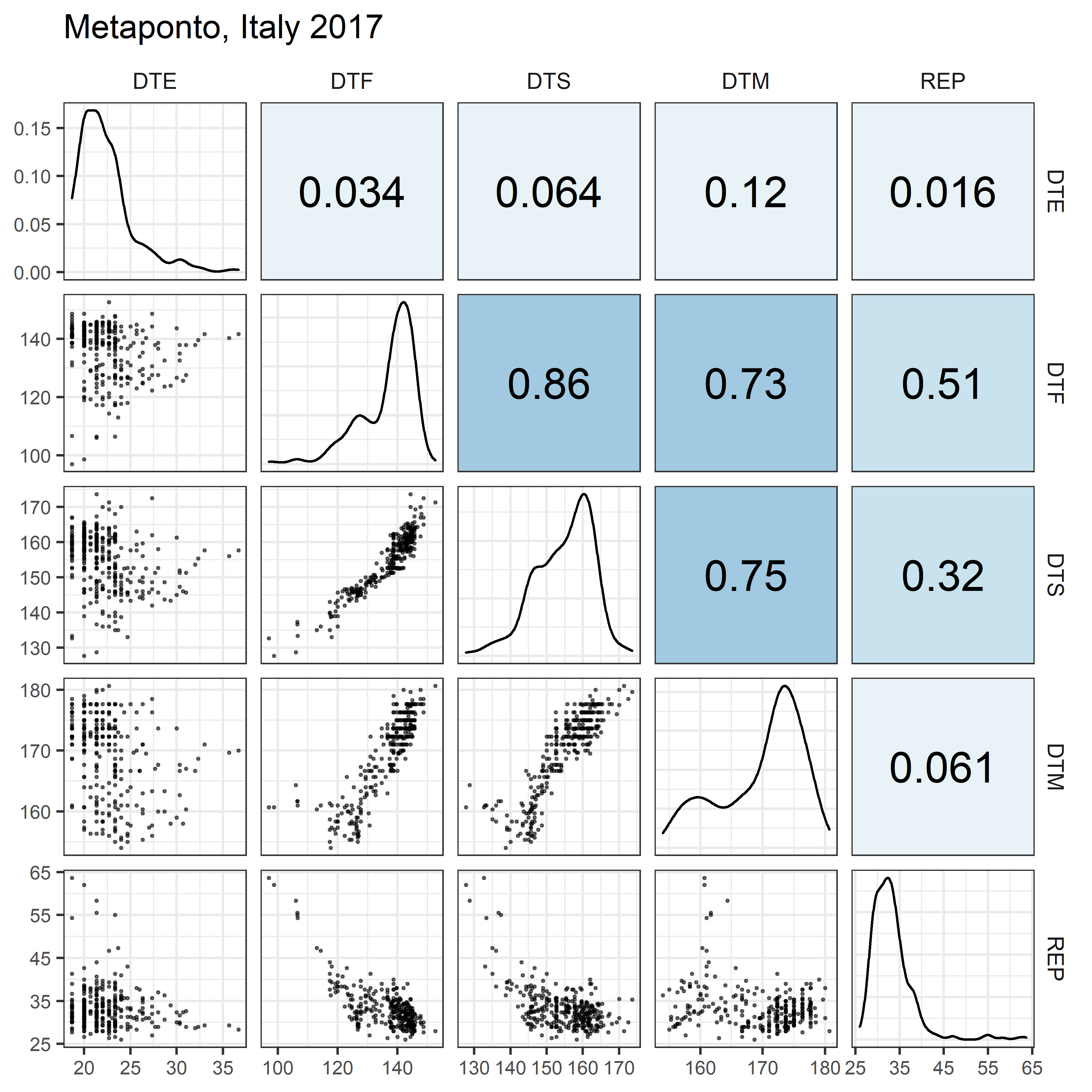
# Prep data
xx <- dd %>%
left_join(select(ff, Expt, MacroEnv), by = "Expt") %>%
mutate(DTE = ifelse(Location == "Cordoba, Spain", NA, DTE))
x1 <- xx %>% filter(MacroEnv == "Temperate")
x2 <- xx %>% filter(MacroEnv == "South Asia")
x3 <- xx %>% filter(MacroEnv == "Mediterranean")
# Create plotting functions
my_lower <- function(data, mapping, cols = colors_Expt, ...) {
ggplot(data = data, mapping = mapping) +
geom_point(alpha = 0.5, size = 0.3, aes(color = Expt)) +
scale_color_manual(values = cols) +
theme_bw() +
theme(axis.text = element_text(size = 7.5))
}
my_middle <- function(data, mapping, cols = colors_Expt, ...) {
ggplot(data = data, mapping = mapping) +
geom_density(alpha = 0.5) +
scale_color_manual(name = NULL, values = cols) +
scale_fill_manual(name = NULL, values = cols) +
guides(color = F, fill = guide_legend(nrow = 3, byrow = T)) +
theme_bw() +
theme(axis.text = element_text(size = 7.5))
}
# See: https://github.com/ggobi/ggally/issues/139
my_upper <- function(data, mapping, color = I("black"), sizeRange = c(1,5), ...) {
# Prep data
x <- eval_data_col(data, mapping$x)
y <- eval_data_col(data, mapping$y)
#
r2 <- cor(x, y, method = "pearson", use = "complete.obs")^2
rt <- format(r2, digits = 2)[1]
cex <- max(sizeRange)
tt <- as.character(rt)
# plot the cor value
p <- ggally_text(label = tt, mapping = aes(), color = color,
xP = 0.5, yP = 0.5, size = 6, ... ) + theme_bw()
# Create color palette
corColors <- RColorBrewer::brewer.pal(n = 10, name = "RdBu")[2:9]
if (r2 <= -0.9) { corCol <- alpha(corColors[1], 0.5)
} else if (r2 >= -0.9 & r2 <= -0.6) { corCol <- alpha(corColors[2], 0.5)
} else if (r2 >= -0.6 & r2 <= -0.3) { corCol <- alpha(corColors[3], 0.5)
} else if (r2 >= -0.3 & r2 <= 0) { corCol <- alpha(corColors[4], 0.5)
} else if (r2 >= 0 & r2 <= 0.3) { corCol <- alpha(corColors[5], 0.5)
} else if (r2 >= 0.3 & r2 <= 0.6) { corCol <- alpha(corColors[6], 0.5)
} else if (r2 >= 0.6 & r2 <= 0.9) { corCol <- alpha(corColors[7], 0.5)
} else { corCol <- alpha(corColors[8], 0.5) }
# Plot
p <- p +
theme(panel.background = element_rect(fill = corCol),
panel.grid.major = element_blank(),
panel.grid.minor = element_blank())
p
}
# Plot Correlations for each Expt
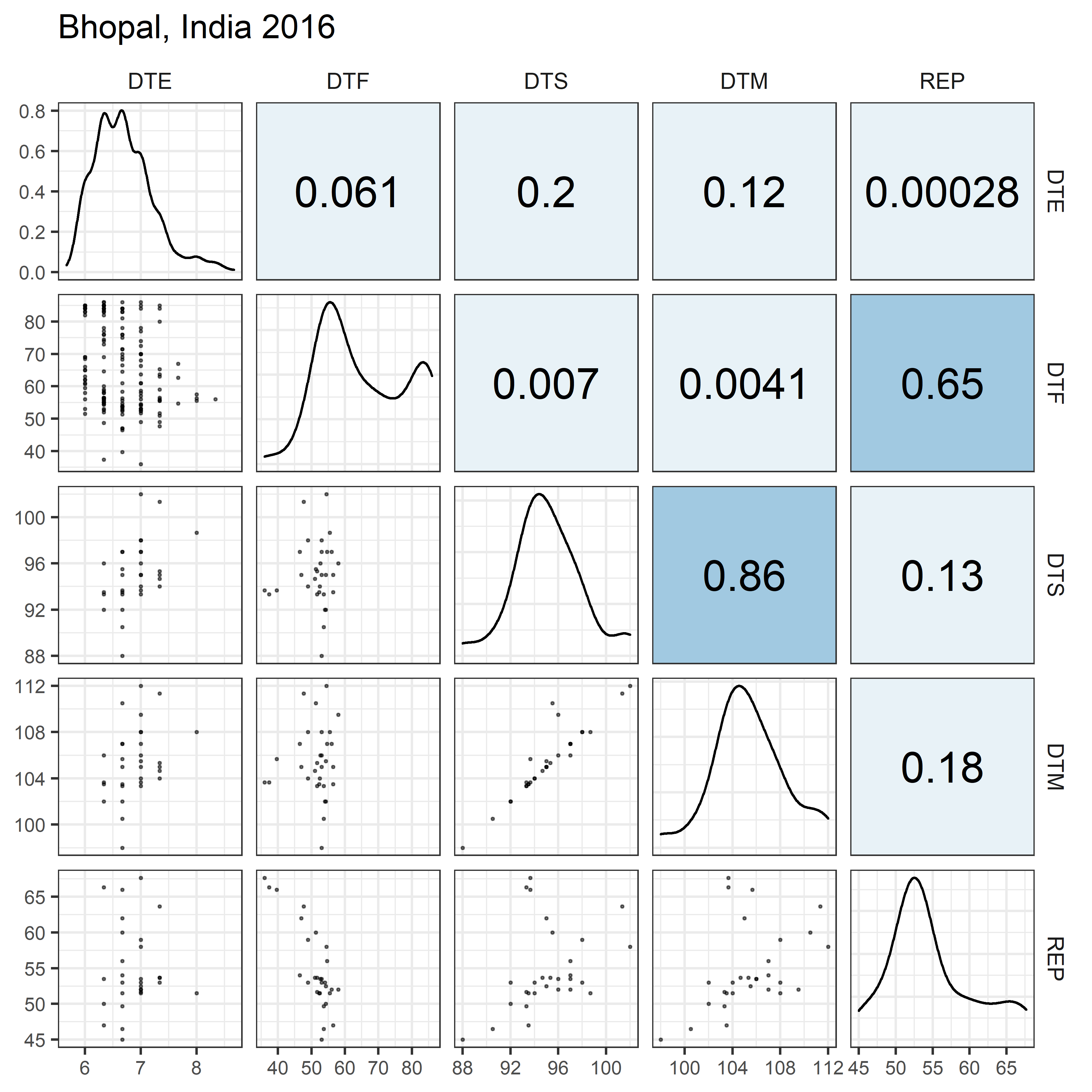
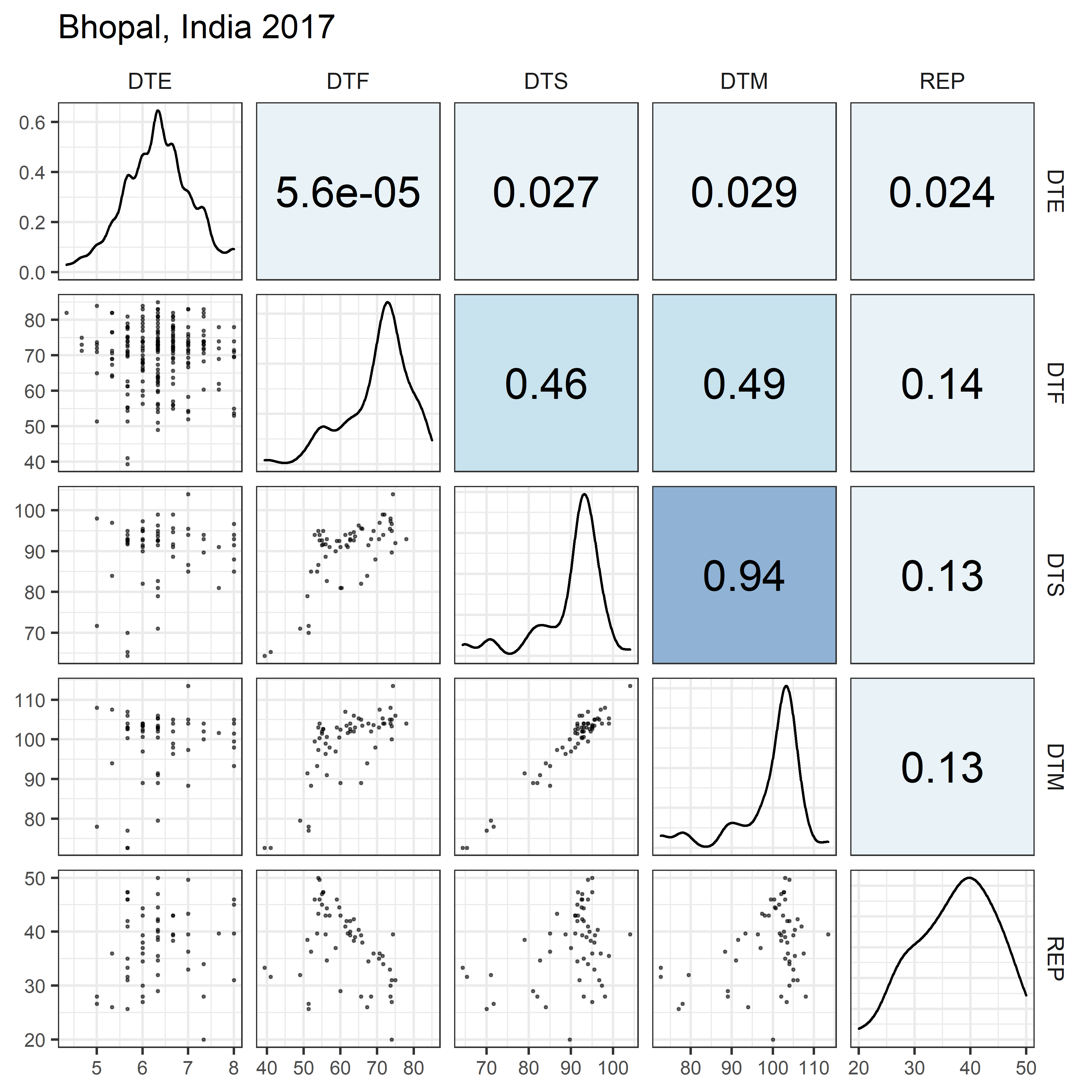
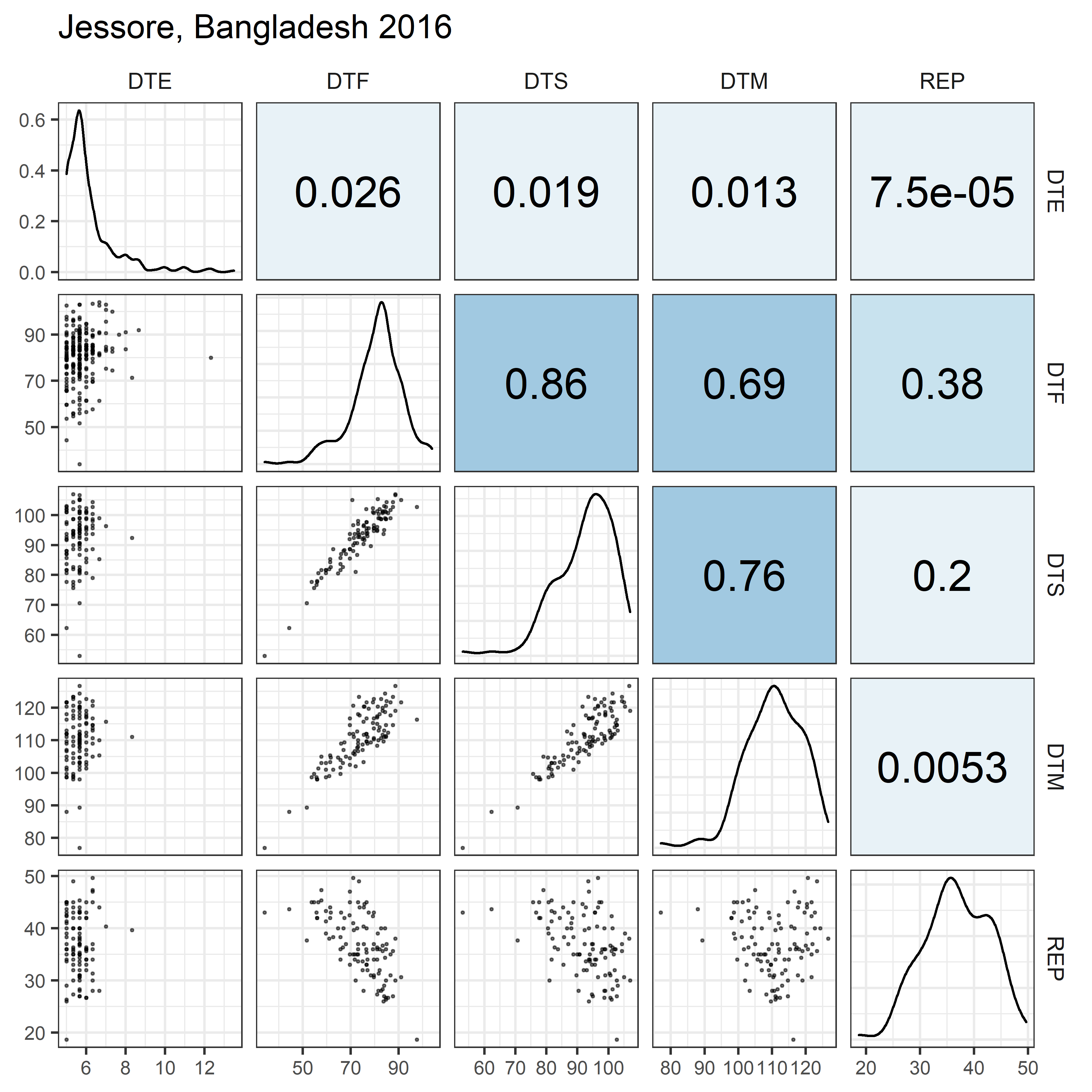
for(i in 1:length(names_Expt)) {
mp <- ggpairs(xx %>% filter(Expt == names_Expt[i]),
columns = c("DTE", "DTF", "DTS", "DTM", "REP"),
upper = list(continuous = my_upper),
diag = list(continuous = my_middle),
lower = list(continuous = wrap(my_lower, cols = "black")),
title = names_Expt[i]) +
theme(strip.background = element_rect(fill = "White"))
ggsave(paste0("Additional/Corr/Corr_", str_pad(i, 2, "left", "0"),
"_", names_ExptShort[i], ".png"),
mp, width = 6, height = 6, dpi = 600)
}
# Plot (a) Temperate
mp1 <- ggpairs(x1, columns = c("DTE", "DTF", "DTS", "DTM", "REP"),
aes(color = Expt, fill = Expt),
upper=list(continuous = my_upper),
diag =list(continuous = wrap(my_middle, cols = colors_Expt[1:6])),
lower=list(continuous = wrap(my_lower, cols = colors_Expt[1:6])),
title = "(a) Temperate",
legend = c(2,2)) +
theme(strip.background = element_rect(fill = "White"),
legend.position = "bottom")
ggsave("Additional/Corr/Corr_Temperate.png", mp1, width = 6, height = 6, dpi = 600)
# Plot (b) South Asia
mp2 <- ggpairs(x2, columns = c("DTE", "DTF", "DTS", "DTM", "REP"),
aes(color = Expt, fill = Expt),
upper = list(continuous = my_upper),
diag = list(continuous = wrap(my_middle, cols = colors_Expt[7:12])),
lower = list(continuous = wrap(my_lower, cols = colors_Expt[7:12])),
title = "(b) South Asia",
legend = c(2,2)) +
theme(strip.background = element_rect(fill = "White"),
legend.position = "bottom")
ggsave("Additional/Corr/Corr_SouthAsia.png", mp2, width = 6, height = 6, dpi = 600)
# Plot (c) Mediterranean
mp3 <- ggpairs(x3, columns = c("DTE", "DTF", "DTS", "DTM", "REP"),
aes(color = Expt, fill = Expt),
upper = list(continuous = my_upper),
diag = list(continuous = wrap(my_middle, cols = colors_Expt[13:18])),
lower = list(continuous = wrap(my_lower, cols = colors_Expt[13:18])),
title = "(c) Mediterranean",
legend = c(2,2)) +
theme(strip.background = element_rect(fill = "White"),
legend.position = "bottom")
ggsave("Additional/Corr/Corr_Mediterranean.png", mp3, width = 6, height = 6, dpi = 600)
# Plot All
mp4 <- ggpairs(xx, columns = c("DTE", "DTF", "DTS", "DTM", "REP"),
aes(color = ExptShort, fill = ExptShort),
upper = list(continuous = my_upper),
diag = list(continuous = my_middle),
lower = list(continuous = my_lower),
title = "ALL",
legend = c(2,2)) +
theme(strip.background = element_rect(fill = "White"),
legend.position = "bottom")
ggsave("Additional/Corr/Corr_All.png", mp4, width = 6, height = 6, dpi = 600)PCA
Figure 3: PCA Clusters
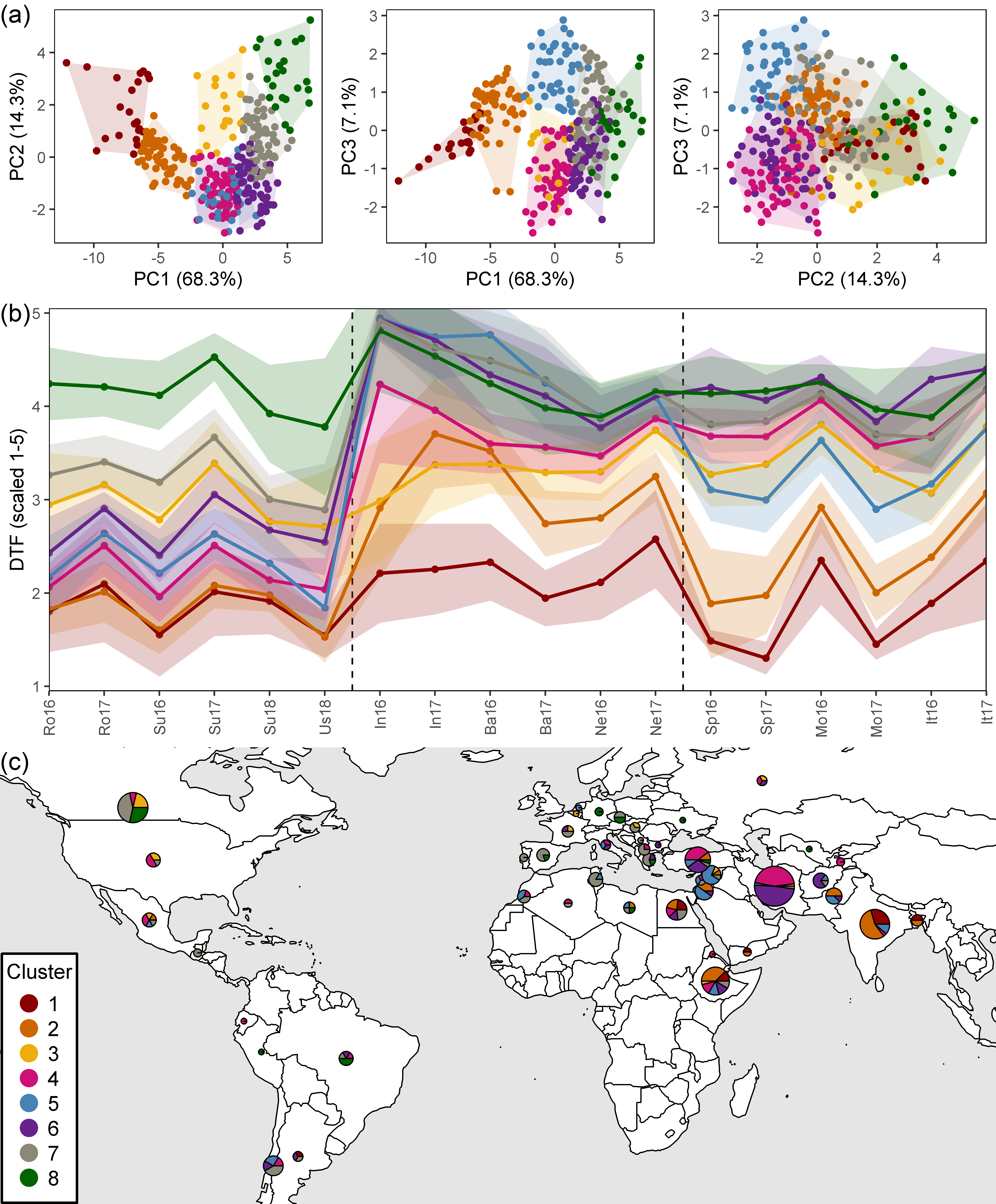
Figure 3: Clustering of a lentil (Lens culinaris Medik.) diversity panel based days from sowing to flower (DTF). (a) Principal Component Analysis on DTF, scaled from 1-5, and hierarchical k-means clustering into eight groups. (b) Mean scaled DTF (1-5) for each cluster group across all field trials: Rosthern, Canada 2016 and 2017 (Ro16, Ro17), Sutherland, Canada 2016, 2017 and 2018 (Su16, Su17, Su18), Central Ferry, USA 2018 (Us18), Metaponto, Italy 2016 and 2017 (It16, It17), Marchouch, Morocco 2016 and 2017 (Mo16, Mo17), Cordoba, Spain 2016 and 2017 (Sp16, Sp17), Bhopal, India 2016 and 2017 (In16, In17), Jessore, Bangladesh 2016 and 2017 (Ba16, Ba17), Bardiya, Nepal 2016 and 2017 (Ne16, Ne17). Shaded areas represent one standard deviation from the mean. Dashed, vertical bars separate temperate, South Asian and Mediterranean macro-environments. (c) Composition of cluster groups in genotypes by country of origin. Pie size is relative to the number of genotypes originating from that country.
# Prep data
xx <- dd %>%
  select(Entry, Expt, DTF2_scaled) %>%
  spread(Expt, DTF2_scaled)
xx <- xx %>% column_to_rownames("Entry") %>% as.matrix()
# PCA
mypca <- PCA(xx, ncp = 10, graph = F)
# Heirarcical clustering
mypcaH <- HCPC(mypca, nb.clust = 8, graph = F)
perc <- round(mypca[[1]][,2], 1)
x1 <- mypcaH[[1]] %>% rownames_to_column("Entry")
x2 <- mypca[[3]]$coord %>% as.data.frame() %>% rownames_to_column("Entry")
pca <- left_join(x1, x2, by = "Entry") %>%
  mutate(Entry = as.numeric(Entry)) %>%
  left_join(select(ldp, Entry, Name, Origin), by = "Entry") %>%
  left_join(select(ct, Origin=Country, Region), by = "Origin") %>%
  select(Entry, Name, Origin, Region, Cluster=clust,
         PC1=Dim.1, PC2=Dim.2, PC3=Dim.3, PC4=Dim.4, PC5=Dim.5,
         PC6=Dim.6, PC7=Dim.7, PC8=Dim.8, PC9=Dim.9, PC10=Dim.10)
# Save data
write.csv(pca, "data/data_pca_results.csv", row.names = F)
# Prep data
x2 <- dd %>%
  left_join(select(pca, Entry, Cluster), by = "Entry") %>%
  group_by(Expt, ExptShort, Cluster) %>%
  summarise(mean = mean(DTF2_scaled, na.rm = T),
            sd = sd(DTF2_scaled, na.rm = T)) %>%
  ungroup() %>%
  mutate(ClusterNum = plyr::mapvalues(Cluster, as.character(1:8), summary(pca$Cluster)))
x3 <- pca %>%
  count(Cluster) %>%
  mutate(Cluster = factor(Cluster, levels = rev(levels(Cluster))), y = n/2)
for(i in 2:nrow(x3)) { x3$y[i] <- sum(x3$n[1:(i-1)]) + (x3$n[i]/2) }
# Plot (a) PCA 1v2
find_hull <- function(df) df[chull(df[,"PC1"], df[,"PC2"]), ]
polys <- plyr::ddply(pca, "Cluster", find_hull) %>% mutate(Cluster = factor(Cluster))
mp1.1 <- ggplot(pca) +
  geom_polygon(data = polys, alpha = 0.15, aes(x = PC1, y = PC2, fill = Cluster)) +
  geom_point(aes(x = PC1, y = PC2, colour = Cluster)) +
  scale_fill_manual(values = colors) +
  scale_color_manual(values = colors) +
  theme_AGL +
  theme(legend.position = "none", panel.grid = element_blank()) +
  labs(x = paste0("PC1 (", perc[1], "%)"),
       y = paste0("PC2 (", perc[2], "%)"))
# Plot (a) PCA 1v3
find_hull <- function(df) df[chull(df[,"PC1"], df[,"PC3"]), ]
polys <- plyr::ddply(pca, "Cluster", find_hull) %>% mutate(Cluster = factor(Cluster))
mp1.2 <- ggplot(pca) +
  geom_polygon(data = polys, alpha = 0.15, aes(x = PC1, y = PC3, fill = Cluster)) +
  geom_point(aes(x = PC1, y = PC3, colour = Cluster)) +
  scale_fill_manual(values = colors) +
  scale_color_manual(values = colors) +
  theme_AGL +
  theme(legend.position = "none", panel.grid = element_blank()) +
  labs(x = paste0("PC1 (", perc[1], "%)"),
       y = paste0("PC3 (", perc[3], "%)"))
# Plot (a) PCA 2v3
find_hull <- function(df) df[chull(df[,"PC2"], df[,"PC3"]), ]
polys <- plyr::ddply(pca, "Cluster", find_hull) %>% mutate(Cluster = factor(Cluster))
mp1.3 <- ggplot(pca) +
  geom_polygon(data = polys, alpha = 0.15, aes(x = PC2, y = PC3, fill = Cluster)) +
  geom_point(aes(x = PC2, y = PC3, colour = Cluster)) +
  scale_fill_manual(values = colors) +
  scale_color_manual(values = colors) +
  theme_AGL +
  theme(legend.position = "none", panel.grid = element_blank()) +
  labs(x = paste0("PC2 (", perc[2], "%)"),
       y = paste0("PC3 (", perc[3], "%)"))
# Append
mp1 <- ggarrange(mp1.1, mp1.2, mp1.3, nrow = 1, ncol = 3, hjust = 0)
# Plot (b) DTF
mp2 <- ggplot(x2, aes(x = ExptShort, y = mean, group = Cluster)) +
  geom_point(aes(color = Cluster)) +
  geom_vline(xintercept = 6.5,  lty = 2) +
  geom_vline(xintercept = 12.5, lty = 2) +
  geom_ribbon(aes(ymin = mean - sd, ymax = mean + sd, fill = Cluster),
              alpha = 0.2, color = NA) +
  geom_line(aes(color = Cluster), size = 1) +
  scale_color_manual(values = colors) +
  scale_fill_manual(values = colors) +
  coord_cartesian(ylim = c(0.95,5.05), expand = F) +
  theme_AGL +
  theme(axis.text.x = element_text(angle = 45, hjust = 1),
        legend.position = "none", panel.grid = element_blank()) +
  labs(y = "DTF (scaled 1-5)", x = NULL)
#
ggsave("Additional/Temp/Temp_F03_1.png", mp1, width = 8, height =   1*6/2.5, dpi = 600)
ggsave("Additional/Temp/Temp_F03_2.png", mp2, width = 8, height = 1.5*6/2.5, dpi = 600)
# Plot (c)
xx <- ldp %>% left_join(select(pca, Entry, Cluster), by = "Entry")
xx <- xx %>%
  filter(!Origin %in% c("ICARDA","USDA","Unknown")) %>%
  group_by(Origin, Cluster) %>%
  summarise(Count = n()) %>%
  spread(Cluster, Count) %>%
  left_join(select(ct, Origin=Country, Lat, Lon), by = "Origin") %>%
  ungroup() %>%
  as.data.frame()
xx[is.na(xx)] <- 0
invisible(png("Additional/Temp/Temp_F03_3.png", width = 4800, height = 2200, res = 600))
par(mai = c(0,0,0,0), xaxs = "i", yaxs = "i")
mapPies(dF = xx, nameX = "Lon", nameY = "Lat", zColours = colors,
          nameZs = c("1","2","3","4","5","6","7","8"), lwd = 1,
          xlim = c(-140,110), ylim = c(0,20), addCatLegend = F,
          oceanCol = "grey90", landCol = "white", borderCol = "black")
legend(-139.5, 15.5, title = "Cluster", legend = 1:8, col = colors,
       pch = 16, cex = 1, pt.cex = 2, box.lwd = 2)
invisible(dev.off())
# Append (a), (b) and (c)
im1 <- image_read("Additional/Temp/Temp_F03_1.png") %>%
  image_annotate("(a)", size = 120, location = "+0+0")
im2 <- image_read("Additional/Temp/Temp_F03_2.png") %>%
  image_annotate("(b)", size = 120, location = "+0+0")
im3 <- image_read("Additional/Temp/Temp_F03_3.png") %>%
  image_annotate("(c)", size = 120, location = "+0+0")
im <- image_append(c(im1, im2, im3), stack = T)
image_write(im, "Figure_03.png")
Additional Figure 5: PCA Plot
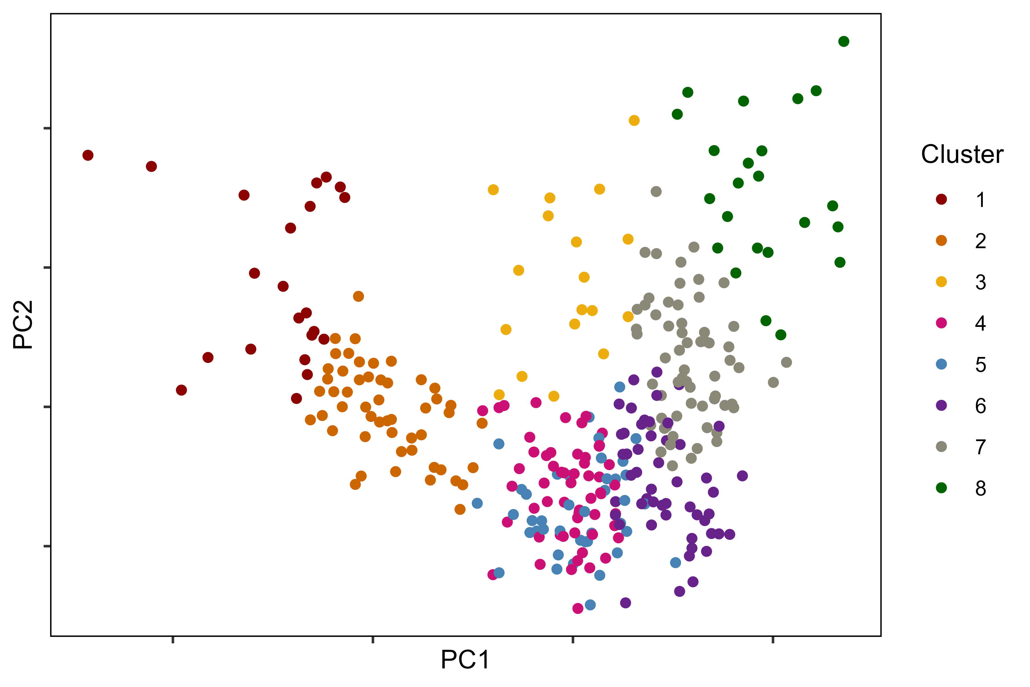
# Prep data
xx <- read.csv("data/data_pca_results.csv") %>%
  mutate(Cluster = factor(Cluster),
         PC2 = PC2*2.5, PC3 = PC3*2.5,
         myColors = plyr::mapvalues(Cluster, 1:8, colors))
# Plot png
mp <- ggplot(xx, aes(x = PC1, y = PC2, color = Cluster)) +
  scale_color_manual(values = colors) +
  geom_point() +
  theme_AGL +
  theme(panel.grid.major.x = element_blank(),
        panel.grid.major.y = element_blank(),
        axis.text = element_blank())
ggsave("Additional/Additional_Figure_05.png", mp, width = 6, height = 4, dpi = 600)
# Plot html
mp <- plot_ly(xx, x = ~PC1, y = ~PC2, z = ~PC3,
              color = ~Cluster, colors = colors,
              text = ~paste(Entry, "|", Name, "\nOrigin:", Origin)) %>%
  add_markers()
saveWidget(mp, file="Additional/Additional_Figure_05.html")
# Prep data
xx <- read.csv("data/data_pca_results.csv") %>%
mutate(Cluster = factor(Cluster),
PC2 = PC2*2.5, PC3 = PC3*2.5,
myColors = plyr::mapvalues(Cluster, 1:8, colors))
# Create plotting function
ggPCA <- function(x = xx, i = 1) {
# Plot
par(mar=c(1.5, 2.5, 1.5, 0.5))
scatter3D(x = x$PC1, y = x$PC3, z = x$PC2, pch = 16, cex = 0.75,
col = alpha(colors,0.8), colvar = as.numeric(x$Cluster), colkey = F,
col.grid = "gray90", bty = "u",
theta = i, phi = 15,
#ticktype = "detailed", cex.lab = 1, cex.axis = 0.5,
xlab = "PC1", ylab = "PC3", zlab = "PC2", main = "LDP - DTF")
}
# Plot each angle
for (i in seq(0, 360, by = 2)) {
png(paste0("Additional/PCA/PCA_", str_pad(i, 3, pad = "0"), ".png"),
width = 1000, height = 1000, res = 300)
ggPCA(xx, i)
dev.off()
}
# Create animation
lf <- list.files("Additional/PCA")
mp <- image_read(paste0("Additional/PCA/", lf))
animation <- image_animate(mp, fps = 10)
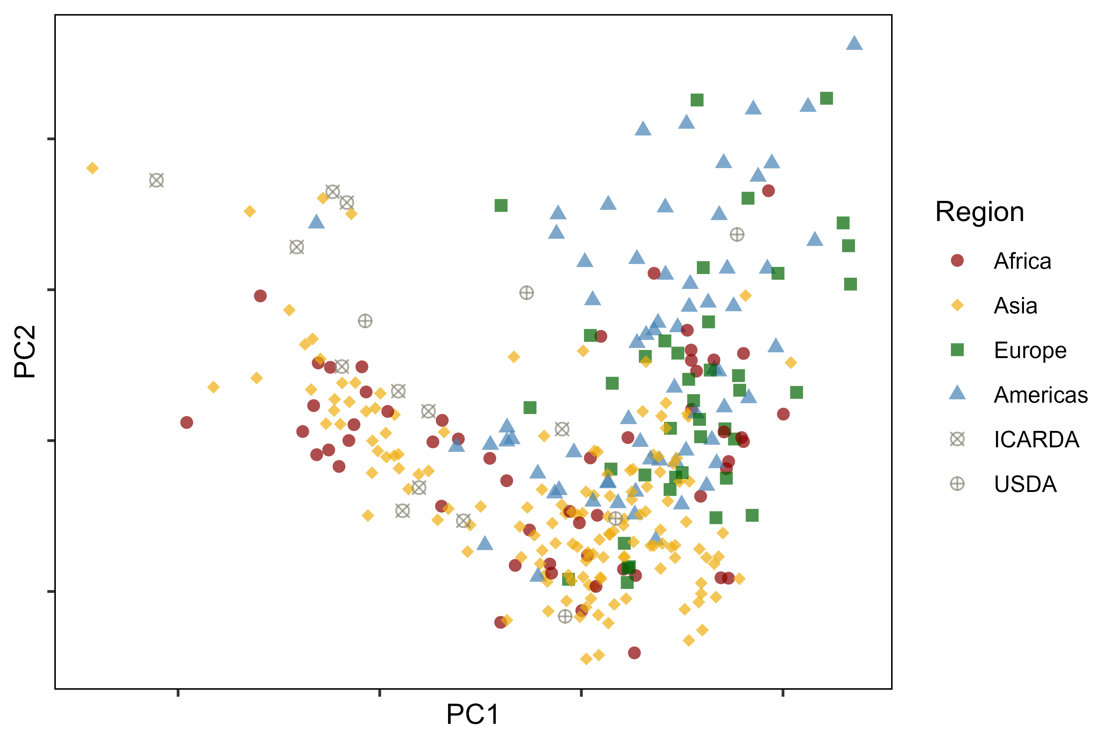
image_write(animation, "Additional/Animation_PCA.gif")Additional Figure 6: PCA by Region
# Prep data
levs <- c("Africa", "Asia", "Europe", "Americas", "ICARDA", "USDA")
xx <- read.csv("data/data_pca_results.csv") %>%
  filter(Origin != "Unknown") %>%
  mutate(Cluster = factor(Cluster),
         PC2 = PC2*2.5, PC3 = PC3*2.5,
         Origin = as.character(Origin),
         Region = as.character(Region),
         Region = ifelse(Origin %in% levs[5:6], Origin, Region),
         Region = factor(Region, levels = levs))
# Plot png
mp <- ggplot(xx, aes(x = PC1, y = PC2, color = Region, shape = Region)) +
  geom_point(alpha = 0.7, size = 2) +
  scale_color_manual(values = colors[c(1,3,8,5,7,7)]) +
  scale_shape_manual(values = c(16,18,15,17,13,10)) +
  theme_AGL +
  theme(panel.grid.major.x = element_blank(),
        panel.grid.major.y = element_blank(),
        axis.text = element_blank())
ggsave("Additional/Additional_Figure_06.png", mp, width = 6, height = 4, dpi = 600)
# Plot html
mp <- plot_ly(xx, x = ~PC1, y = ~PC2, z = ~PC3, color = ~Region,
              colors = colors[c(1,3,8,5,7,7)],
              text = ~paste(Entry, "|", Name, "\nOrigin:", Origin,
                            "\nCluster:", Cluster)) %>%
  add_markers()
saveWidget(mp, file="Additional/Additional_Figure_06.html")
Additional Figure 7: DTF By Cluster
# Prep data
x1 <- read.csv("data/data_pca_results.csv") %>%
  mutate(Cluster = factor(Cluster))
x2 <- c("India", "Bangladesh", "Ethiopia", "Pakistan",
        "Jordan", "Iran", "Turkey", "Syria", "Chile",
        "Spain", "Czech Republic", "Canada" )
xx <- dd %>%
  left_join(ldp, by = "Entry") %>%
  filter(ExptShort %in% c("Ro17", "Ba17", "Ne17", "It17"), Origin != "Unknown") %>%
  left_join(select(x1, Entry, Cluster), by = "Entry") %>%
  mutate(Origin = factor(Origin, levels = unique(Origin)[rev(order(unique(Origin)))])) %>%
  filter(Origin %in% x2) %>%
  mutate(Origin = factor(Origin, levels = x2))
# Plot
mp <- ggplot(xx, aes(y = DTF2, x = Origin, group = Expt)) +
  geom_quasirandom(aes(color = Cluster)) +
  facet_grid(Location + Year ~ ., scales = "free_y") +
  scale_color_manual(values = colors) +
  theme_AGL +
  theme(legend.position = "top",
        panel.grid.major.x = element_blank(),
        axis.text.x = element_text(angle = 45, hjust = 1)) +
  guides(colour = guide_legend(nrow = 1, override.aes = list(size = 3))) +
  labs(y = "Days from sowing to flower")
ggsave("Additional/Additional_Figure_07.png", mp, width = 5, height = 7, dpi = 600)
Additional Figure 8: Cluster Origins
# Prep data
xx <- read.csv("data/data_pca_results.csv") %>%
  mutate(Cluster = factor(Cluster))
xx <- ldp %>%
  left_join(select(xx, Entry, Cluster), by = "Entry")
x1 <- xx %>% filter(Origin != "ICARDA") %>%
  group_by(Origin, Cluster) %>%
  summarise(Count = n()) %>%
  spread(Cluster, Count) %>%
  left_join(select(ct, Origin=Country, Lat, Lon), by = "Origin") %>%
  ungroup() %>%
  as.data.frame()
x1[is.na(x1)] <- 0
# Plot
mp <- ggplot(xx, aes(x = Origin, fill = Cluster)) +
  geom_bar(stat = "count") +
  facet_grid(. ~ Cluster, scales = "free", space = "free") +
  scale_fill_manual(values = colors) +
  theme_AGL +
  theme(legend.position = "none",
        panel.grid.major.x = element_blank(),
        axis.text.x = element_text(angle = 45, hjust = 1)) +
  labs(y = "Count", x = NULL)
ggsave("Additional/Additional_Figure_08.png", width = 16, height = 4, dpi = 600)
Additional Figure 9: LDP Origins By Cluster
# Prep data
xx <- read.csv("data/data_pca_results.csv") %>%
  mutate(Cluster = factor(Cluster))
xx <- ldp %>%
  select(Entry, Name, Lat, Lon, Origin) %>%
  left_join(select(xx, Entry, Cluster), by = "Entry") %>%
  left_join(select(ct, Origin=Country, cLat=Lat, cLon=Lon), by = "Origin") %>%
  mutate(Lat = ifelse(is.na(Lat), cLat, Lat),
         Lon = ifelse(is.na(Lon), cLon, Lon),
         Lat = ifelse(duplicated(Lat), jitter(Lat, 1, 1), Lat),
         Lon = ifelse(duplicated(Lon), jitter(Lon, 1, 1), Lon),
         Size = 1)
# Plot png
invisible(png("Additional/Additional_Figure_09.png",
              width = 7200, height = 4200, res = 600))
par(mai = c(0,0,0,0), xaxs = "i", yaxs = "i")
mapBubbles(dF = xx, nameX = "Lon", nameY = "Lat", nameZColour = "Cluster",
           pch = 20, nameZSize = "Size", symbolSize = 0.5,
           xlim = c(-140,110), ylim = c(0,20),
           colourPalette = colors[1:8], addColourLegend = F, addLegend = F,
           oceanCol = "grey90", landCol = "white", borderCol = "black")
legend(-139.5, 15.5, title = "Cluster", legend = 1:8, col = colors,
       pch = 16, cex = 1.75, pt.cex = 3, box.lwd = 2)
invisible(dev.off())
# Plot html
pal <- colorFactor(colors, domain = 1:8)
mp <- leaflet() %>%
  addProviderTiles(providers$CartoDB.Positron) %>%
  addCircles(lng = xx$Lon, lat = xx$Lat, weight = 10,
                   color = pal(xx$Cluster), opacity = 1, fillOpacity = 1,
                   popup = paste(xx$Entry,"|",xx$Name,"\nCluster:",xx$Cluster)) %>%
  addLegend("bottomleft", pal = pal, values = xx$Cluster,
            title = "Cluster", opacity = 1)
saveWidget(mp, file="Additional/Additional_Figure_09.html")
Modeling DTF
Additional Figures: Entry Regressions
myfills <- alpha(c("darkgreen", "darkorange3", "darkblue"), 0.5)
mymin <- min(rr$RDTF, na.rm = T)
mymax <- max(rr$RDTF, na.rm = T)
mp <- list()
for(i in 1:324) {
  xx <- rr %>%
    filter(Entry == i) %>%
    left_join(select(ff, Expt, MacroEnv, T_mean, P_mean), by = "Expt") %>%
    mutate(myfill = MacroEnv)
  x1 <- xx %>% filter(MacroEnv != "South Asia")
  x2 <- xx %>% filter(MacroEnv != "Temperate")
  x3 <- xx %>% filter(MacroEnv != "Mediterranean")
  figlab <- paste("Entry", str_pad(i, 3, "left", "0"), "|", unique(xx$Name))
  # Plot (a) 1/f = a + bT
  mp1 <- ggplot(xx, aes(x = T_mean, y = RDTF)) +
    geom_point(aes(shape = MacroEnv, color = MacroEnv)) +
    geom_smooth(data = x1, method = "lm", se = F, color = "black", lty = 3) +
    geom_smooth(data = x2, method = "lm", se = F, color = "black") +
    scale_y_continuous(sec.axis = dup_axis(~ 1/., name = NULL, breaks = c(35,50,100,150)),
                       trans = "reverse", breaks = c(0.01,0.02,0.03), limits = c(mymax, mymin)) +
    scale_x_continuous(breaks = c(11,13,15,17,19,21)) +
    scale_shape_manual(name = "Macro-environment", values = c(16,15,17)) +
    scale_color_manual(name = "Macro-environment", values = myfills) +
    theme_AGL +
    labs(title = figlab, y = "1 / DTF",
         x = expression(paste("Temperature (", degree, "C)", sep="")))
  # Plot (b) 1/f = a + cP
  mp2 <- ggplot(xx, aes(x = P_mean, y = RDTF)) +
    geom_point(aes(shape = MacroEnv, color = MacroEnv)) +
    geom_smooth(data = x1, method = "lm", se = F, color = "black", lty = 3) +
    geom_smooth(data = x3, method = "lm", se = F, color = "black") +
    scale_y_continuous(sec.axis = dup_axis(~ 1/., name="DTF", breaks = c(35,50,100,150)),
                       trans = "reverse", breaks = c(0.01,0.02,0.03), limits = c(mymax, mymin)) +
    scale_x_continuous(breaks = c(11,12,13,14,15,16)) +
    scale_shape_manual(name = "Macro-environment", values = c(16,15,17)) +
    scale_color_manual(name = "Macro-environment", values = myfills) +
    theme_AGL +
    labs(title = "", y = NULL,x = "Photoperiod (hours)")
  #
  mp[[i]] <- ggarrange(mp1, mp2, ncol = 2, common.legend = T, legend = "bottom")
  ggsave(paste0("Additional/Entry_TP/TP_Entry_", str_pad(i, 3, pad = "0"), ".png"),
         mp[[i]], width = 8, height = 4, dpi = 600)
}
pdf("Additional/pdf_TP.pdf", width = 8, height = 4)
for(i in 1:324) { print(mp[[i]]) }
dev.off()
Additional Figures: PhotoThermal Plane
# Prep data
xx <- rr %>%
  filter(!is.na(RDTF)) %>%
  left_join(select(ff, Expt, T_mean, P_mean, MacroEnv), by = "Expt")
# Create plotting function
ggPTplane <- function(x, i) {
  x1 <- x %>% filter(Entry == i)
  x <- x1$T_mean
  y <- x1$P_mean
  z <- x1$RDTF
  fit <- lm(z ~ x + y)
  # Create PhotoThermal plane
  fitp <- predict(fit)
  grid.lines <- 12
  x.p <- seq(min(x), max(x), length.out = grid.lines)
  y.p <- seq(min(y), max(y), length.out = grid.lines)
  xy <- expand.grid(x = x.p, y = y.p)
  z.p <- matrix(predict(fit, newdata = xy), nrow = grid.lines, ncol = grid.lines)
  pchs <- plyr::mapvalues(x1$Expt, names_Expt, c(rep(16,6), rep(15,6), rep(17,6))) %>%
    as.character() %>% as.numeric()
  # Plot with regression plane
  par(mar=c(1.5, 2.5, 1.5, 0.5))
  scatter3D(x, y, z, pch = pchs, cex = 2, main = unique(x1$Name),
    col = alpha(c("darkgreen", "darkorange3", "darkblue"),0.5),
    colvar = as.numeric(x1$MacroEnv), colkey = F, col.grid = "gray90",
    bty = "u", theta = 40, phi = 25, ticktype = "detailed",
    cex.lab = 1, cex.axis = 0.5, zlim = c(0.005,0.03),
    xlab = "Temperature", ylab = "Photoperiod", zlab = "1 / DTF",
    surf = list(x = x.p, y = y.p, z = z.p, col = "black", facets = NA, fit = fitp) )
}
# Plot each Entry
for (i in 1:324) {
  png(paste0("Additional/Entry_3D/3D_Entry_", str_pad(i, 3, pad = "0"), ".png"),
      width = 1000, height = 1000, res = 300)
  ggPTplane(xx, i)
  dev.off()
}
# Create PDF
pdf("Additional/pdf_3D.pdf")
par(mar=c(1.5, 2.5, 1.5, 0.5))
for (i in 1:324) {
  ggPTplane(xx, i)
}
dev.off()
#
# Plot ILL 5888 & ILL 4400 & Laird
xx <- xx %>% mutate(Name = gsub(" AGL", "", Name))
for (i in c(235, 94, 128)) {
  png(paste0("Additional/Temp/3D_Entry_", str_pad(i, 3, pad = "0"), ".png"),
      width = 2000, height = 2000, res = 600)
  ggPTplane(xx, i)
  dev.off()
}
# Create animation
xx <- read.csv("data/model_t+p_coefs.csv") %>% arrange(b, c)
lf <- list.files("Additional/Entry_3D")[xx$Entry]
mp <- image_read(paste0("Additional/Entry_3D/", lf))
animation <- image_animate(mp, fps = 10)
image_write(animation, "Additional/Animation_3D.gif")
Supplemental Figure 4: Regressions
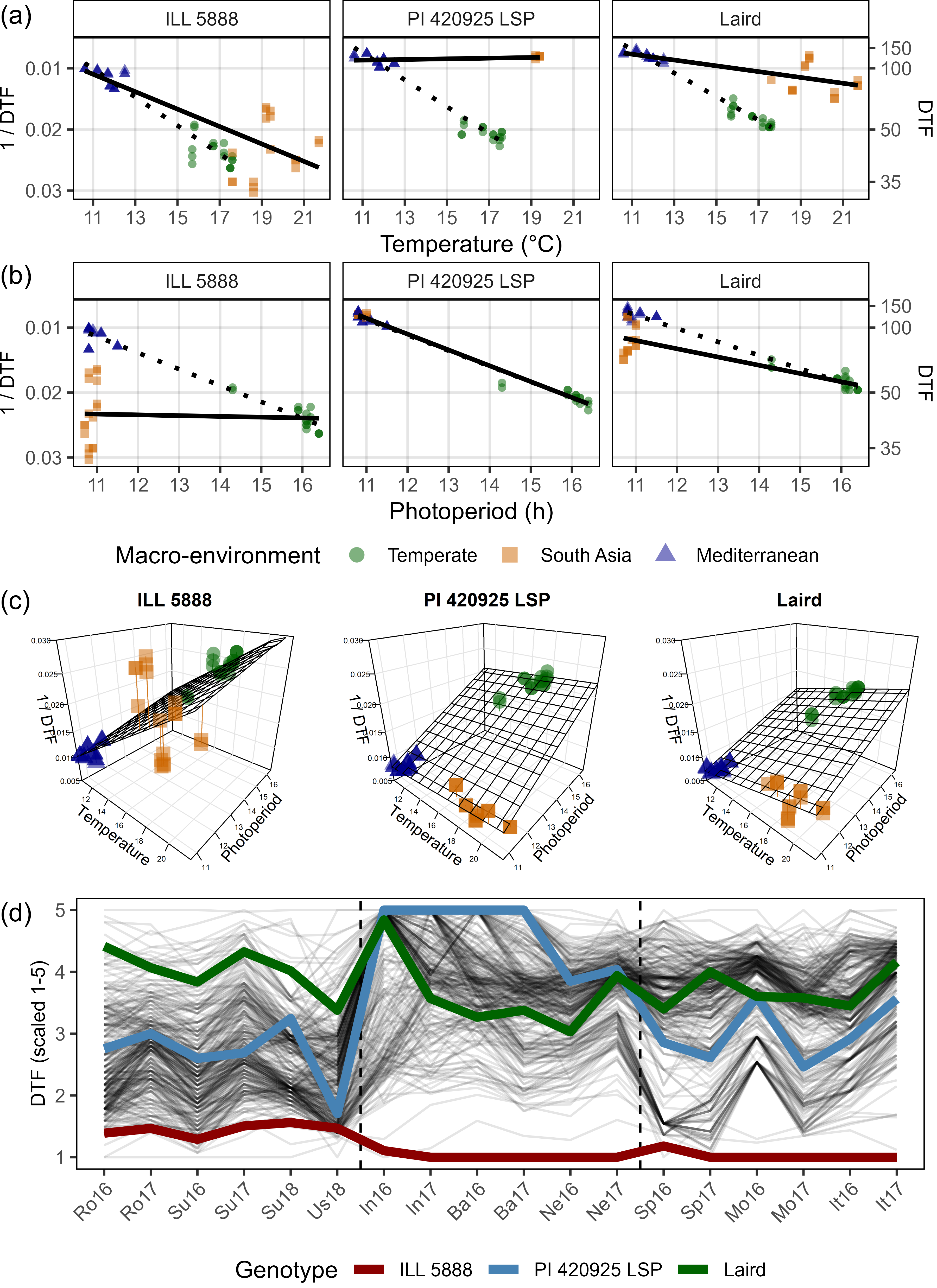
Figure S4: Effects of mean temperature and photoperiod on the rate of progress towards flowering (1 / DTF) in three contrasting selected genotypes. (a) Effect of temperature on 1 / DTF, (b) effect of photoperiod on 1 / DTF, and (c) effect of temperature and photoperiod on 1 / DTF modelled using equation 1. For (a) and (b), solid lines represent regressions among locations of relatively constant photoperiod or temperature, respectively, while dotted lines indicate a break in the assumption of constant photoperiod or temperature, respectively, across environments (see Figure 1). (d) Scaled DTF (1-5) of each genotype (grey lines) across all site-years with ILL5888, PI 420925 LSP and Laird highlighted according to their corresponding cluster group, 1, 5 and 8 respectively. ILL 5888 is an early maturing, genotype from Bangladesh. PI 420925 LSP is a landrace from Jordan with medium maturity. Laird is a late maturing, Canadian cultivar.
# Prep data
myfills <- alpha(c("darkgreen", "darkorange3", "darkblue"), 0.5)
yy <- c("ILL 5888 AGL", "PI 420925 LSP AGL",  "Laird AGL")
xx <- rr %>%
  filter(Name %in% yy, !is.na(DTF)) %>%
  left_join(select(ff, Expt, MacroEnv, T_mean, P_mean), by = "Expt") %>%
  mutate(Name = gsub(" AGL", "", Name), myfill = MacroEnv,
         Name = factor(Name, levels = gsub(" AGL", "", yy)))
x1 <- xx %>% filter(MacroEnv != "South Asia")
x2 <- xx %>% filter(MacroEnv != "Temperate")
x3 <- xx %>% filter(MacroEnv != "Mediterranean")
# Plot (a) 1/f = a + bT
mp1 <- ggplot(xx, aes(x = T_mean, y = RDTF)) +
  geom_point(aes(shape = MacroEnv, color = MacroEnv)) +
  geom_smooth(data = x1, method = "lm", se = F, color = "black", lty = 3) +
  geom_smooth(data = x2, method = "lm", se = F, color = "black") +
  scale_y_continuous(trans = "reverse", breaks = c(0.01,0.02,0.03),
                     sec.axis = dup_axis(~ 1/., name = "DTF", breaks = c(35,50,100,150))) +
  scale_x_continuous(breaks = c(11,13,15,17,19,21)) +
  scale_shape_manual(name = "Macro-environment", values = c(16,15,17)) +
  scale_color_manual(name = "Macro-environment", values = myfills) +
  theme_AGL + facet_grid(. ~ Name) +
  theme(axis.title.y = element_text(size = 9),
        plot.margin = unit(c(0,0,0,0), "cm")) +
  guides(colour = guide_legend(override.aes = list(size = 3))) +
  labs(y = "1 / DTF", x = expression(paste("Temperature (", degree, "C)", sep = "")))
# Plot (b) 1/f = a + cP
mp2 <- ggplot(xx, aes(x = P_mean, y = RDTF)) +
  geom_point(aes(shape = MacroEnv, color = MacroEnv)) +
  geom_smooth(data = x1, method = "lm", se = F, color = "black", lty = 3) +
  geom_smooth(data = x3, method = "lm", se = F, color = "black") +
  scale_y_continuous(trans = "reverse", breaks = c(0.01,0.02,0.03),
                     sec.axis = dup_axis(~ 1/., name="DTF", breaks = c(35,50,100,150))) +
  scale_x_continuous(breaks = c(11,12,13,14,15,16)) +
  scale_shape_manual(name = "Macro-environment", values = c(16,15,17)) +
  scale_color_manual(name = "Macro-environment", values = myfills) +
  theme_AGL + facet_grid(. ~ Name) +
  theme(axis.title.y = element_text(size = 9),
        plot.margin = unit(c(0,0,0,0), "cm")) +
  guides(colour = guide_legend(override.aes = list(size = 3))) +
  labs(y = "1 / DTF",x = "Photoperiod (h)")
# Append (a) and (b)
mp <- ggarrange(mp1, mp2, ncol = 1, common.legend = T, legend = "bottom")
ggsave("Additional/Temp/Temp_SF04_1.png", mp, width = 6, height = 3.75, dpi = 600, bg = "white")
# Append (c)s
im1 <- image_read("Additional/Temp/3D_Entry_094.png")
im2 <- image_read("Additional/Temp/3D_Entry_235.png")
im3 <- image_read("Additional/Temp/3D_Entry_128.png")
im <- image_append(c(im1, im2, im3)) %>% image_scale("3600x")
image_write(im, "Additional/Temp/Temp_SF04_2.png")
# Prep data
xx <- dd %>%
  filter(Name %in% yy) %>%
  mutate(Name = gsub(" AGL", "", Name),
         Name = factor(Name, levels = gsub(" AGL", "", yy)))
# Plot D)
mp3 <- ggplot(dd, aes(x = ExptShort, y = DTF2_scaled, group = Name)) +
  geom_line(color = "black", alpha = 0.1) +
  geom_vline(xintercept = 6.5,  lty = 2) +
  geom_vline(xintercept = 12.5, lty = 2) +
  geom_line(data = xx, aes(color = Name), size = 2) +
  scale_color_manual(name = "Genotype", values = colors[c(1,5,8)]) +
  theme_AGL + labs(y = "DTF (scaled 1-5)", x = NULL) +
  theme(legend.position = "bottom",
        legend.margin = unit(c(0,0,0,0), "cm"),
        plot.margin   = unit(c(0,0.2,0,0.5), "cm"),
        panel.grid   = element_blank(),
        axis.title.y = element_text(size = 9),
        axis.text.x  = element_text(angle = 45, hjust = 1))
ggsave("Additional/Temp/Temp_SF04_3.png", mp3, width = 6, height = 2.5, dpi = 600)
# Append (a), (b), C) and D)
im1 <- image_read("Additional/Temp/Temp_SF04_1.png") %>%
  image_annotate("(a)", size = 100, location = "+0+0") %>%
  image_annotate("(b)", size = 100, location = "+0+1000")
im2 <- image_read("Additional/Temp/Temp_SF04_2.png") %>%
  image_annotate("(c)", size = 100)
im3 <- image_read("Additional/Temp/Temp_SF04_3.png") %>%
  image_annotate("(d)", size = 100)
im <- image_append(c(im1, im2, im3), stack = T)
image_write(im, "Supplemental_Figure_04.png")
Modeling DTF - Functions
# Create functions
# Plot Observed vs Predicted
ggModel1 <- function(x, title = NULL, type = 1,
    mymin = min(c(x$DTF,x$Predicted_DTF)) - 2,
    mymax = max(c(x$DTF,x$Predicted_DTF)) + 2 ) {
  x <- x %>% mutate(Flowered = ifelse(is.na(DTF), "Did not Flower", "Flowered"))
  # Prep data
  if(type == 1) {
    myx <- "DTF"; myy <- "Predicted_DTF"
    x <- x %>% filter(!is.na(DTF))
  }
  if(type == 2) {
    myx <- "RDTF"; myy <- "Predicted_RDTF"
    x <- x %>% filter(!is.na(RDTF))
  }
  myPal <- colors_Expt[names_Expt %in% unique(x$Expt)]
  r2 <- round(modelR2(x = x[,myx], y = x[,myy]), 3)
  # Plot
  mp <- ggplot(x) +
    geom_point(aes(x = get(myx), y = get(myy), color = Expt)) +
    geom_abline() +
    geom_label(x = mymin, y = mymax, hjust = 0, vjust = 1, parse = T,
               label = paste("italic(R)^2 == ", r2)) +
    scale_x_continuous(limits = c(mymin, mymax), expand = c(0, 0)) +
    scale_y_continuous(limits = c(mymin, mymax), expand = c(0, 0)) +
    scale_color_manual(name = NULL, values = myPal) +
    guides(colour = guide_legend(override.aes = list(size = 2))) +
    theme_AGL
  if(type == 1) {
    mp <- mp + labs(y = "Predicted DTF (days)", x = "Observed DTF (days)")
  }
  if(type == 2) {
    mp <- mp +
      scale_x_reverse(limits = c(mymax, mymin), expand = c(0, 0)) +
      scale_y_reverse(limits = c(mymax, mymin), expand = c(0, 0)) +
      labs(y = "Predicted RDTF (1/days)", x = "Observed RDTF (1/days)")
  }
  if(!is.null(title)) { mp <- mp + labs(title = title) }
  mp
}
# Facets by Expt
ggModel2 <- function(x, myX = "DTF", myY = "Predicted_DTF", title = NULL,
                       x1 = 30, x2 = 30, y1 = 145, y2 = 120, legend.pos = "bottom") {
  # Prep data
  pca <- read.csv("data/data_pca_results.csv") %>%
    select(Entry, Cluster) %>%
    mutate(Cluster = factor(Cluster))
  x <- x %>%
    filter(!is.na(get(myX))) %>%
    left_join(pca, by = "Entry")
  xf <- x %>%
    group_by(Expt) %>%
    summarise(Mean = mean(DTF)) %>%
    ungroup() %>%
    mutate(r2 = NULL, RMSE = NULL)
  for(i in 1:nrow(xf)) {
    xi <- x %>% filter(Expt == xf$Expt[i])
    xf[i,"r2"]   <- round(modelR2(x = xi[,myX],   y = xi[,myY]), 2)
    xf[i,"RMSE"] <- round(modelRMSE(x = xi[,myX], y = xi[,myY]), 1)
  }
  # Plot
  mp <- ggplot(x, aes(x = get(myX), y = get(myY))) +
    geom_point(aes(color = Cluster), size = 0.75, alpha = 0.7) + geom_abline() +
    geom_text(x = x1, y = y1, color = "black", hjust = 0, vjust = 0, size = 3,
              aes(label = paste("RMSE = ", RMSE, sep = "")), data = xf) +
    geom_text(x = x2, y = y2, color = "black", hjust = 0, vjust = 0, size = 3,
              aes(label = paste("italic(R)^2 == ", r2)), parse = T, data = xf) +
    facet_wrap(Expt ~ ., ncol = 6, labeller = label_wrap_gen(width = 17)) +
    scale_x_continuous(limits = c(min(x[,myX]), max(x[,myX]))) +
    scale_y_continuous(limits = c(min(x[,myX]), max(x[,myX]))) +
    scale_color_manual(values = colors) +
    theme_AGL +
    theme(axis.text.x = element_text(angle = 45, hjust = 1),
          legend.position = legend.pos,
          legend.margin = unit(c(0,0,0,0), "cm"),
          panel.grid = element_blank()) +
    guides(colour = guide_legend(nrow = 1, override.aes = list(size = 3))) +
    labs(y = "Predicted DTF (days)", x = "Observed DTF (days)")
  if(!is.null(title)) { mp <- mp + labs(title = title) }
  mp
}
# R^2 function
modelR2 <- function(x, y) {
  1 - ( sum((x - y)^2, na.rm = T) / sum((x - mean(x, na.rm = T))^2, na.rm = T))
}
# RMSE function
modelRMSE <- function(x, y) {
  sqrt(sum((x-y)^2, na.rm = T) / length(x))
}
\(R^2=1-\frac{SS_{residuals}}{SS_{total}}=1-\frac{\sum (x-y)^2}{\sum (x-\bar{x})}\)
\(RMSE=\frac{\sum (y-x)^2}{n}\)
Modeling DTF (T + P) - All Site-years
###########################
# 1/f = a + bT + cP (All) #
###########################
# Prep data
xx <- rr %>%
  filter(!is.na(RDTF)) %>%
  left_join(select(ff, Expt, T_mean, P_mean), by = "Expt") %>%
  select(Plot, Entry, Name, Rep, Expt, ExptShort, T_mean, P_mean, RDTF, DTF)
mr <- NULL
md <- NULL
mc <- ldp %>% select(Entry, Name) %>%
  mutate(a = NA, b = NA, c = NA, RR = NA, Environments = NA, aP = NA, bP = NA, cP = NA)
# Model
for(i in 1:324) {
  # Prep data
  xri <- xx %>% filter(Entry == i)
  xdi <- xri %>%
    group_by(Entry, Name, Expt, ExptShort) %>%
    summarise_at(vars(DTF, RDTF, T_mean, P_mean), funs(mean), na.rm = T) %>%
    ungroup()
  # Train Model
  mi <- lm(RDTF ~ T_mean + P_mean, data = xri)
  # Predict DTF
  xri <- xri %>% mutate(Predicted_RDTF = predict(mi),
                        Predicted_DTF = 1 / predict(mi))
  xdi <- xdi %>% mutate(Predicted_RDTF = predict(mi, newdata = xdi),
                        Predicted_DTF = 1 / predict(mi, newdata = xdi))
  # Save to table
  mr <- bind_rows(mr, xri)
  md <- bind_rows(md, xdi)
  # Save coefficients
  mc[i,c("a","b","c")] <- mi$coefficients
  # Calculate rr and # of environments used
  mc[i,"RR"] <- 1 - sum((xri$DTF - xri$Predicted_DTF)^2, na.rm = T) /
    sum((xri$Predicted_DTF - mean(xri$DTF, na.rm = T))^2, na.rm = T)
  mc[i,"Environments"] <- length(unique(xri$Expt[!is.na(xri$DTF)]))
  mc[i,"aP"] <- summary(mi)[[4]][1,4]
  mc[i,"bP"] <- summary(mi)[[4]][2,4]
  mc[i,"cP"] <- summary(mi)[[4]][3,4]
}
mr <- mr %>% mutate(Expt = factor(Expt, levels = names_Expt))
md <- md %>% mutate(Expt = factor(Expt, levels = names_Expt))
# Save Results
write.csv(mr, "data/model_t+p.csv",       row.names = F)
write.csv(md, "data/model_t+p_d.csv",     row.names = F)
write.csv(mc, "data/model_t+p_coefs.csv", row.names = F)
#
# Plot Each Entry
mp <- list()
for(i in 1:324) {
  mp1 <- ggModel1(mr %>% filter(Entry == i), paste("Entry", i, "| DTF"),
           mymin = min(c(mr$Predicted_DTF, mr$DTF), na.rm = T),
           mymax = max(c(mr$Predicted_DTF, mr$DTF), na.rm = T))
  mp2 <- ggModel1(mr %>% filter(Entry == i), paste("Entry", i, "| RDTF"), type = 2,
           mymin = min(c(mr$Predicted_RDTF, mr$RDTF)) - 0.001,
           mymax = max(c(mr$Predicted_RDTF, mr$RDTF)) + 0.001)
  mp[[i]] <- ggarrange(mp1, mp2, ncol = 2, common.legend = T, legend = "right")
  fname <- paste0("Additional/entry_model/model_entry_", str_pad(i, 3, pad = "0"), ".png")
  ggsave(fname, mp[[i]], width = 10, height = 4.5, dpi = 600)
}
pdf("Additional/pdf_Model.pdf", width = 10, height = 4.5)
for (i in 1:324) { print(mp[[i]]) }
dev.off()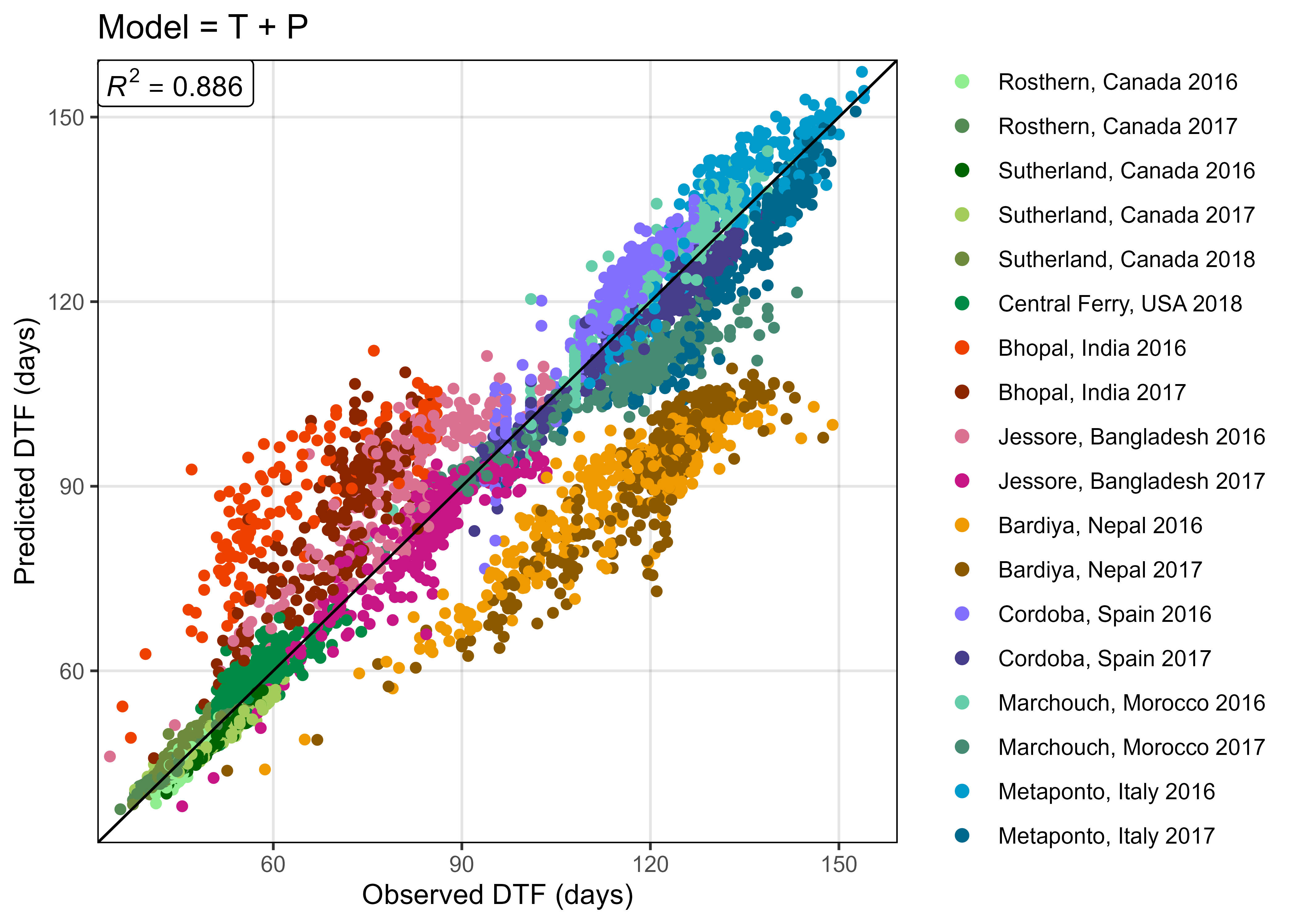
# Prep data
xx <- read.csv("data/model_t+p_d.csv") %>%
  mutate(Expt = factor(Expt, levels = names_Expt))
# Plot Observed vs Predicted
mp <- ggModel1(xx, title = "Model = T + P")
ggsave("Additional/Model/Model_1_1.png", mp, width = 7, height = 5, dpi = 600)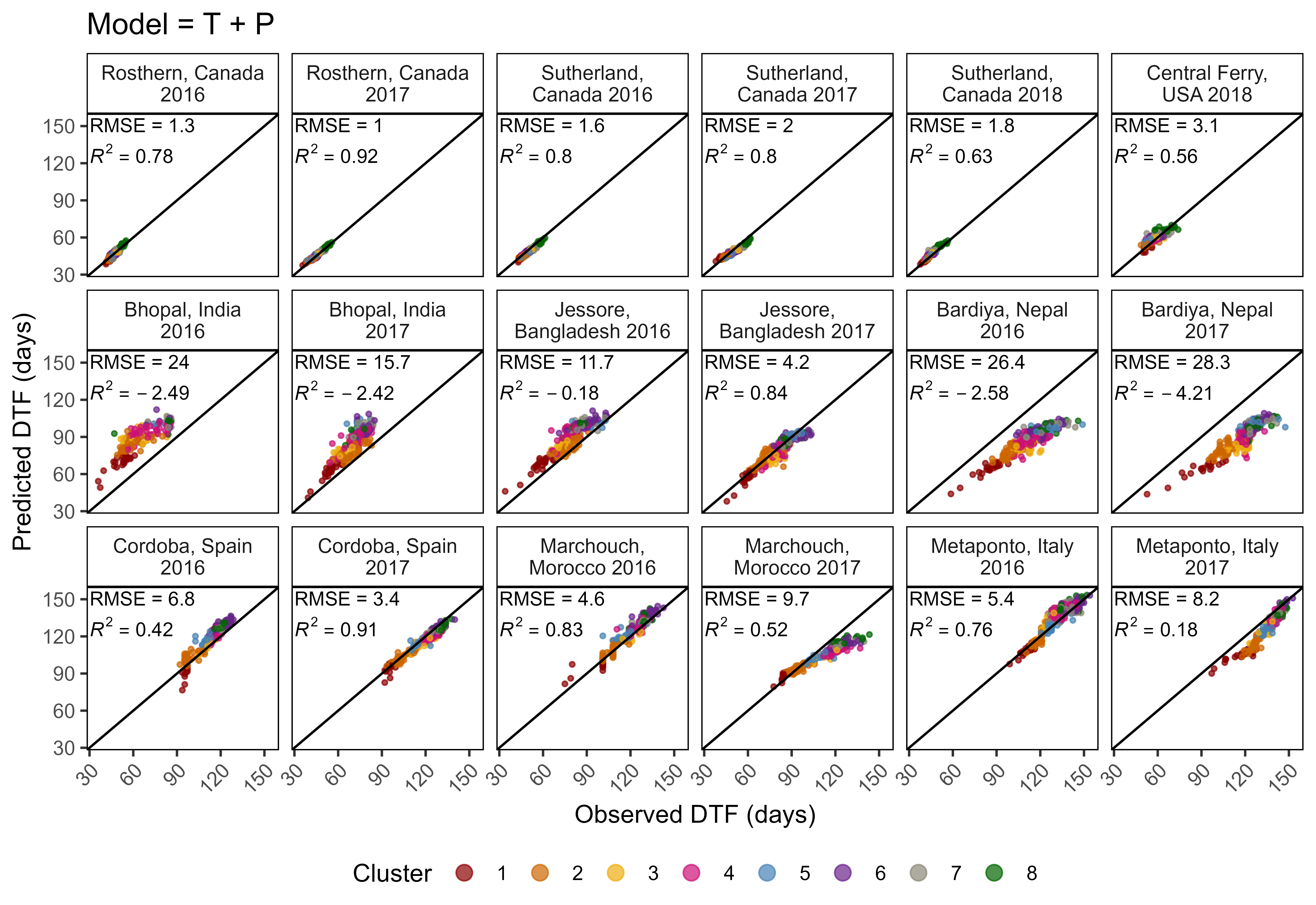
# Plot Observed vs Predicted
mp <- ggModel2(xx, title = "Model = T + P")
ggsave("Additional/Model/Model_2_1.png", mp, width = 8, height = 5.5, dpi = 600)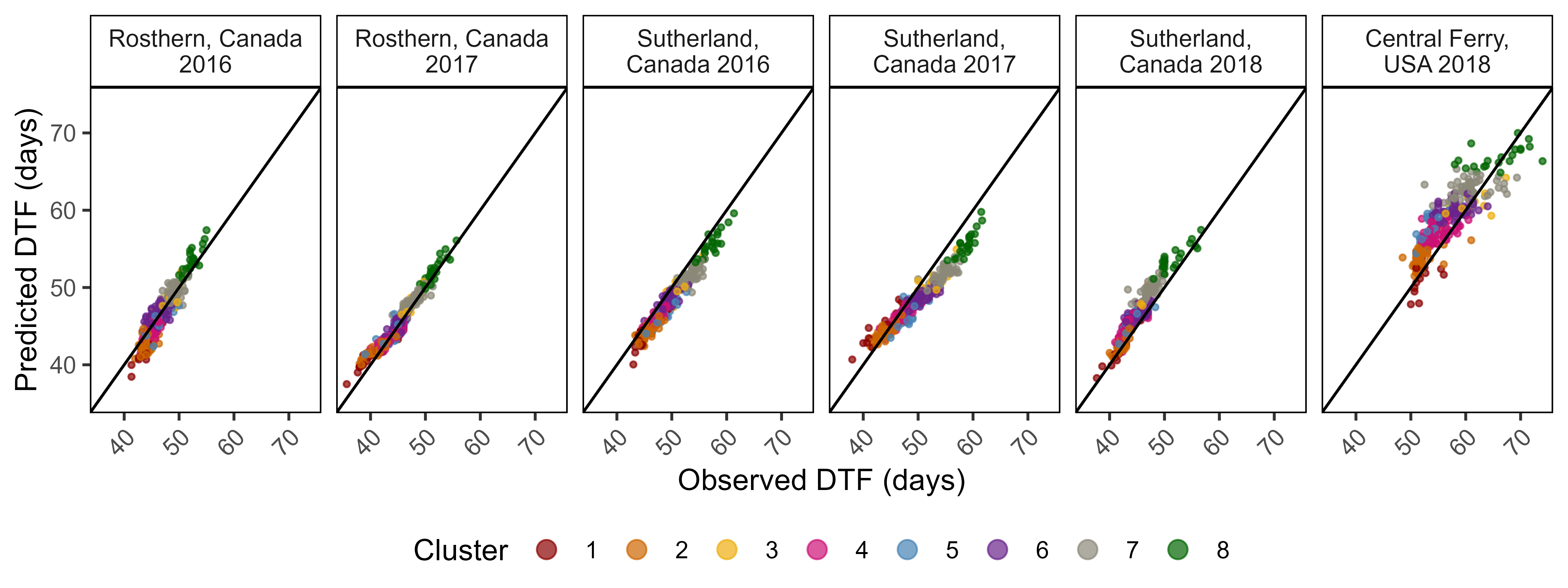
# Plot Observed vs Predicted for Temperate Locations
myexpts <- c("Ro16","Ro17","Su16","Su17","Su18","Us18")
mp <- ggModel2(xx %>% filter(ExptShort %in% myexpts))
ggsave("Additional/Model/Model_3_1.png", mp, width = 8, height = 3, dpi = 600)
Modeling DTF (T x P) - All Site-years
###########################
# 1/f = a + bT + cP (All) #
###########################
# Prep data
xx <- rr %>%
  filter(!is.na(RDTF)) %>%
  left_join(select(ff, Expt, T_mean, P_mean), by = "Expt") %>%
  select(Plot, Entry, Name, Rep, Expt, ExptShort, T_mean, P_mean, RDTF, DTF)
mr <- NULL
md <- NULL
mc <- ldp %>% select(Entry, Name) %>%
  mutate(a = NA, b = NA, c = NA, d = NA, RR = NA, Environments = NA,
         aP = NA, bP = NA, cP= NA, dP = NA)
# Model
for(i in 1:324) {
  # Prep data
  xri <- xx %>% filter(Entry == i)
  xdi <- xri %>%
    group_by(Entry, Name, Expt, ExptShort) %>%
    summarise_at(vars(DTF, RDTF, T_mean, P_mean), funs(mean), na.rm = T) %>%
    ungroup()
  # Train Model
  mi <- lm(RDTF ~ T_mean * P_mean, data = xri)
  # Predict DTF
  xri <- xri %>% mutate(Predicted_RDTF = predict(mi),
                        Predicted_DTF = 1 / predict(mi))
  xdi <- xdi %>% mutate(Predicted_RDTF = predict(mi, newdata = xdi),
                        Predicted_DTF = 1 / predict(mi, newdata = xdi))
  # Save to table
  mr <- bind_rows(mr, xri)
  md <- bind_rows(md, xdi)
  # Save coefficients
  mc[i,c("a","b","c","d")] <- mi$coefficients
  # Calculate rr and # of environments used
  mc[i,"RR"] <- 1 - sum((xri$DTF - xri$Predicted_DTF)^2, na.rm = T) /
    sum((xri$Predicted_DTF - mean(xri$DTF, na.rm = T))^2, na.rm = T)
  mc[i,"Environments"] <- length(unique(xri$Expt[!is.na(xri$DTF)]))
  mc[i,"aP"] <- summary(mi)[[4]][1,4]
  mc[i,"bP"] <- summary(mi)[[4]][2,4]
  mc[i,"cP"] <- summary(mi)[[4]][3,4]
  mc[i,"dP"] <- summary(mi)[[4]][4,4]
}
mr <- mr %>% mutate(Expt = factor(Expt, levels = names_Expt))
md <- md %>% mutate(Expt = factor(Expt, levels = names_Expt))
# Save Results
write.csv(mr, "data/model_txp.csv",       row.names = F)
write.csv(md, "data/model_txp_d.csv",     row.names = F)
write.csv(mc, "data/model_txp_coefs.csv", row.names = F)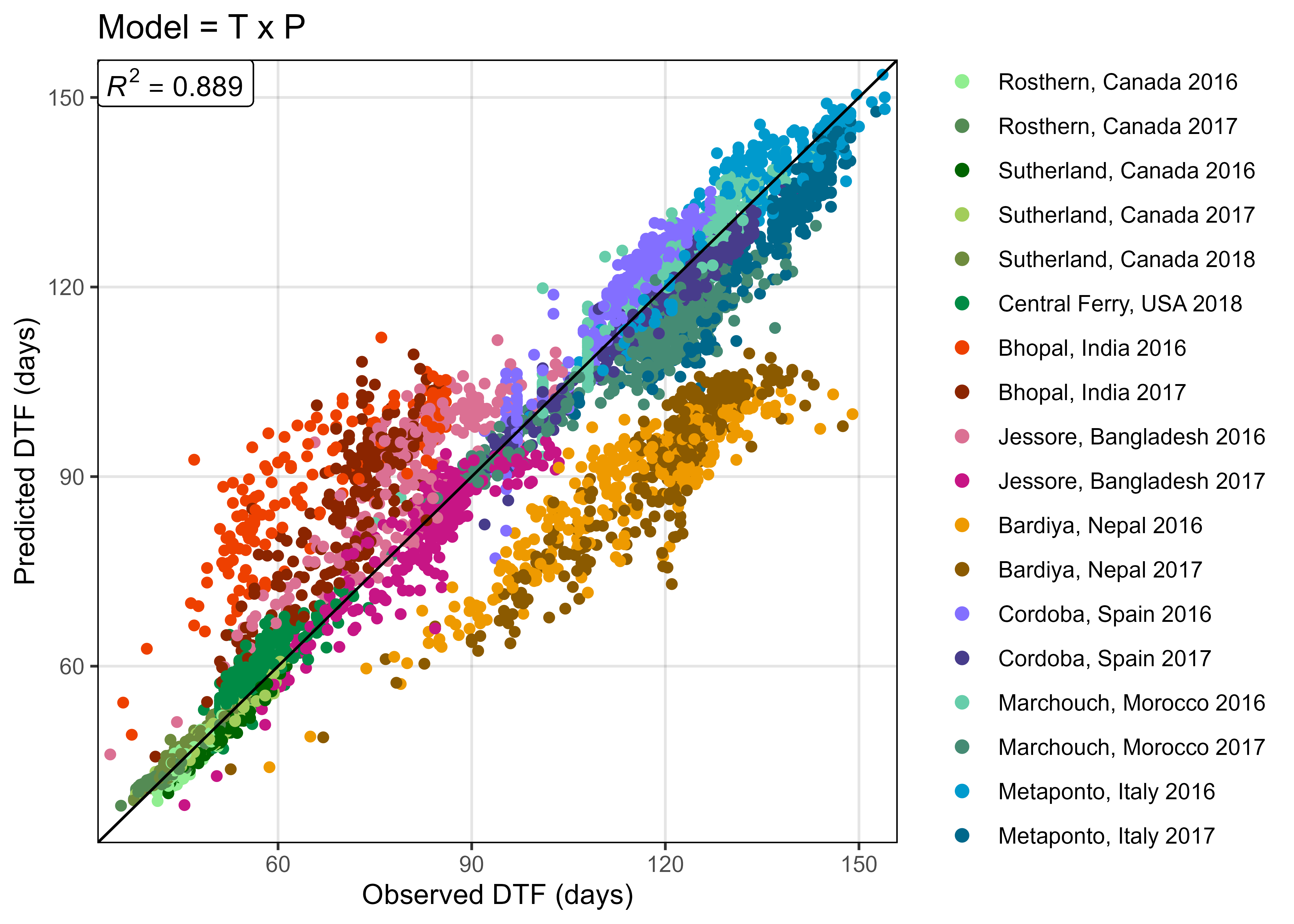
# Prep data
xx <- read.csv("data/model_txp_d.csv") %>%
  mutate(Expt = factor(Expt, levels = names_Expt))
# Plot Observed vs Predicted
mp <- ggModel1(xx, title = "Model = T x P")
ggsave("Additional/Model/Model_1_2.png", mp, width = 7, height = 5, dpi = 600)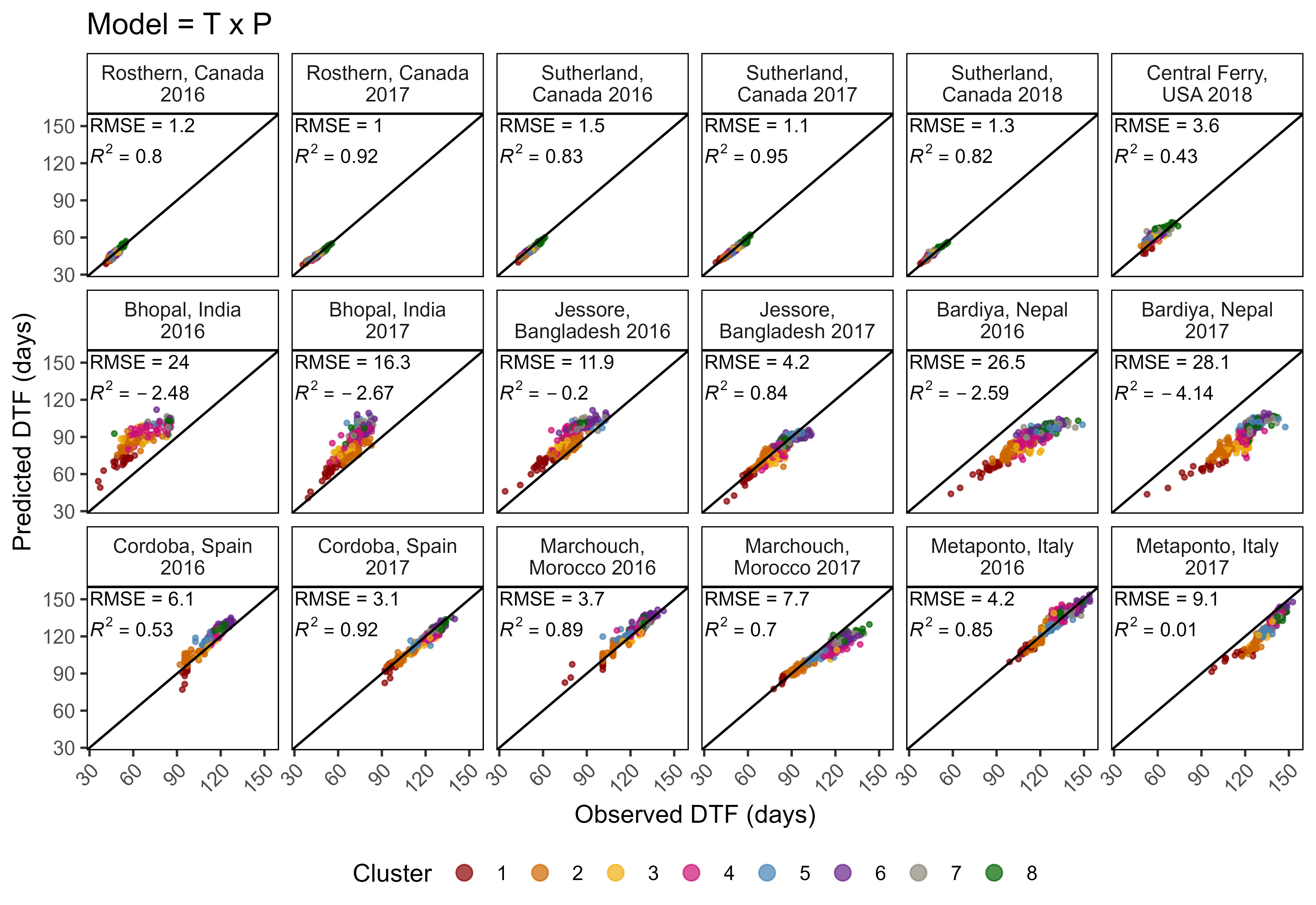
# Plot Observed vs Predicted
mp <- ggModel2(xx, title = "Model = T x P")
ggsave("Additional/Model/Model_2_2.png", mp, width = 8, height = 5.5, dpi = 600)
Supplemental Table 3: Model Constants
Table S3: Values of the constants derived from equations 1 and 2 using data from all site-years, for each of the genotypes used in this study.
# Prep data
x1 <- read.csv("data/model_t+p_coefs.csv")
x2 <- read.csv("data/model_txp_coefs.csv")
xx <- bind_rows(x1, x2) %>%
arrange(Entry) %>%
select(Entry, Name, a, b, c, d, RR, Environments,
a_p.value=aP, b_p.value=bP, c_p.value=cP, d_p.value=dP)
# Save
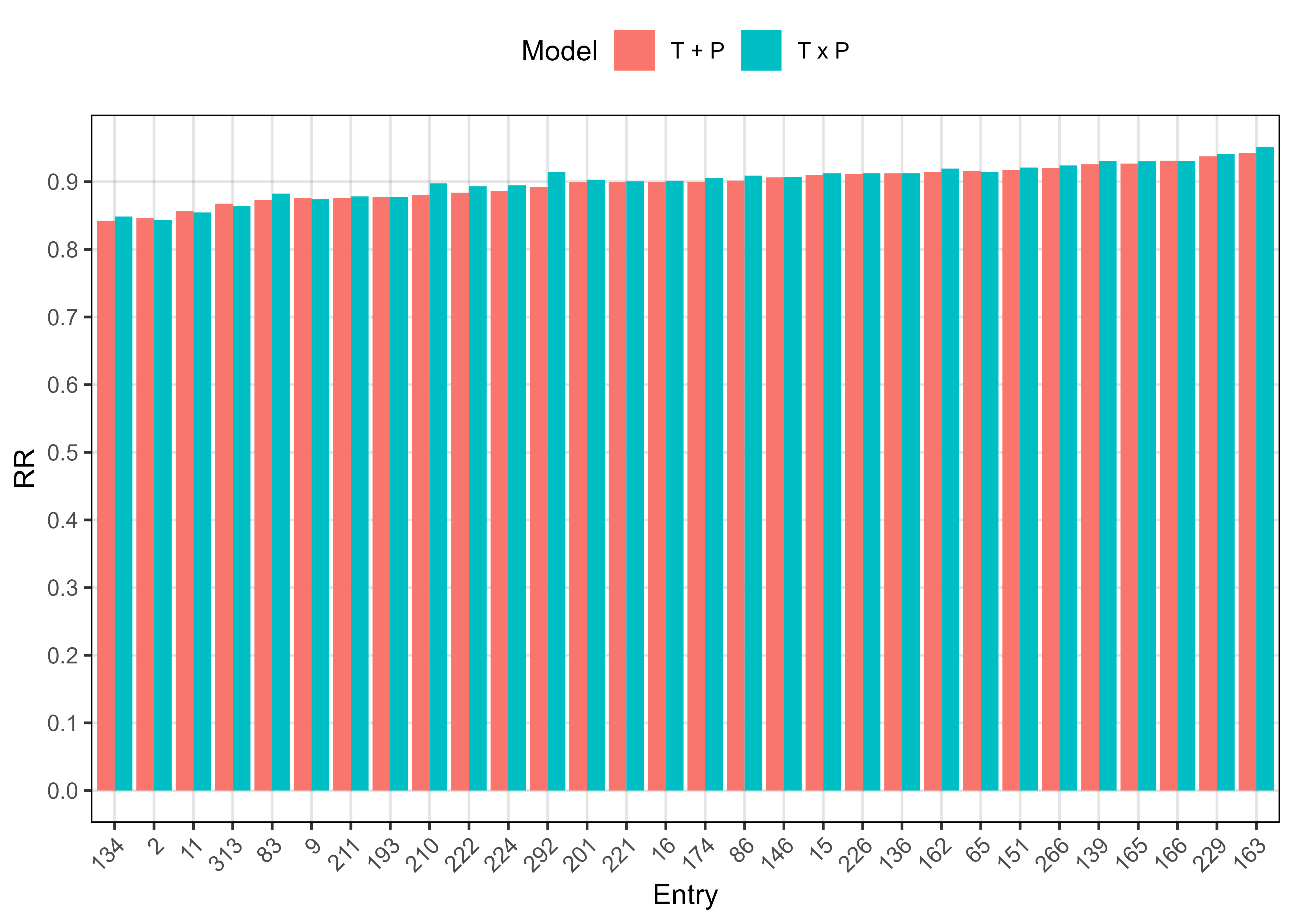
write.csv(xx, "Supplemental_Table_03.csv", na = "", row.names = F)Additional Figure 10: significant T x P interactions
# Prep data
x1 <- read.csv("data/model_t+p_coefs.csv")
x2 <- read.csv("data/model_txp_coefs.csv")
xx <- bind_rows(x1, x2) %>%
  arrange(Entry) %>%
  select(Entry, Name, a, b, c, d, RR)
entries <- x2 %>% filter(dP < 0.05) %>% pull(Entry)
xx <- xx %>% filter(Entry %in% entries)
xx <- xx %>%
  arrange(RR) %>%
  mutate(Entry = factor(Entry, levels = unique(Entry)),
         Model = ifelse(is.na(d), "T + P", "T x P"))
# Plot
mp <- ggplot(xx, aes(x = Entry, y = RR, fill = Model)) +
  geom_bar(stat = "identity", position = "dodge") +
  scale_y_continuous(breaks = seq(0,1,0.1), minor_breaks = seq(0,1,0.01)) +
  theme_AGL +
  theme(legend.position = "top",
        axis.text.x = element_text(angle = 45, hjust = 1))
ggsave("Additional/Additional_Figure_10.png", mp,
       width = 7, height = 5, dpi = 600)
#
length(entries)
[1] 30Supplemental Figure 5: Model T + P vs. T x P
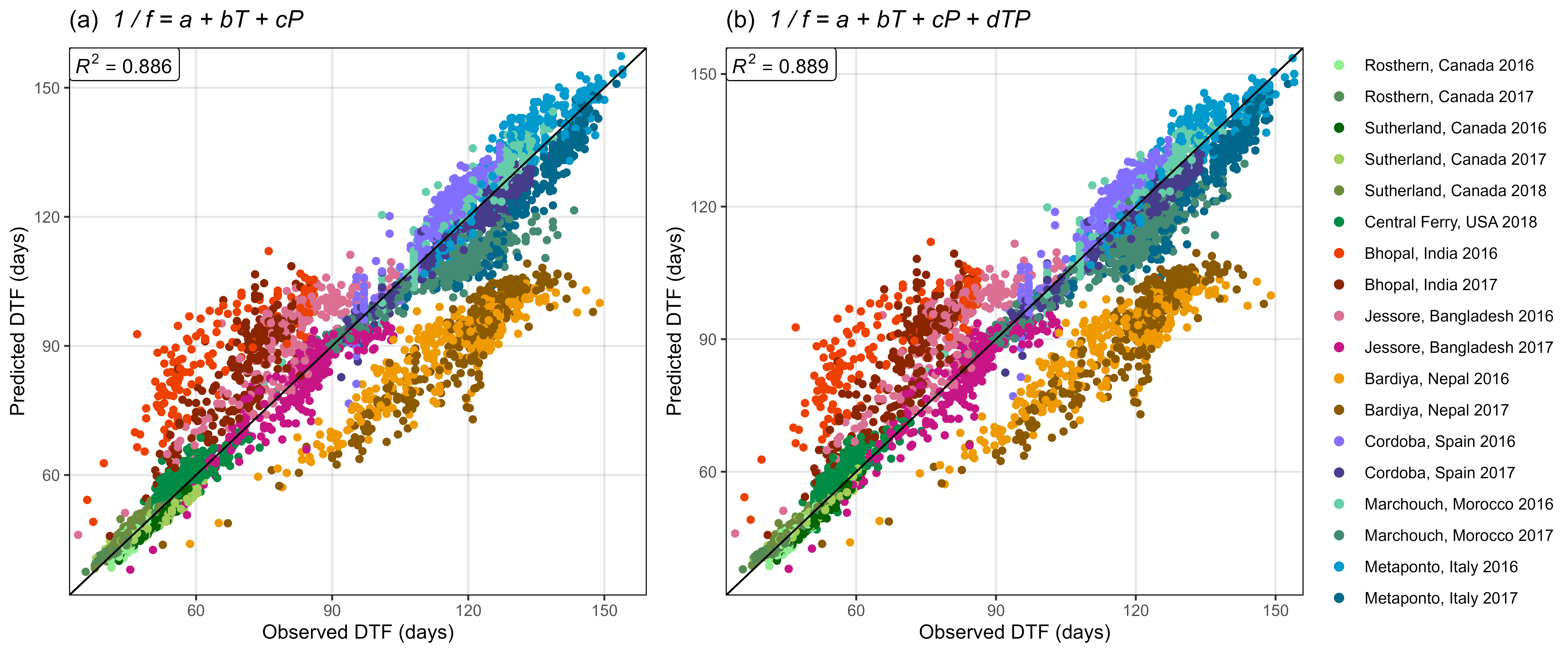
Figure S5: Comparison of observed and predicted values for days from sowing to flowering using (a) equation 1 and (b) equation 2.
# Prep data
xx <- read.csv("data/model_t+p_d.csv") %>%
  mutate(Expt = factor(Expt, levels = names_Expt))
# Plot Observed vs Predicted
mp1 <- ggModel1(xx, title = expression(paste("(a) ", italic(" 1 / f = a + bT + cP"))))
# Prep data
xx <- read.csv("data/model_txp_d.csv") %>%
  mutate(Expt = factor(Expt, levels = names_Expt))
# Plot Observed vs Predicted
mp2 <- ggModel1(xx, title = expression(paste("(b) ", italic(" 1 / f = a + bT + cP + dTP"))))
# Append
mp <- ggarrange(mp1, mp2, ncol = 2, common.legend = T, legend = "right")
ggsave("Supplemental_Figure_05.png", mp, width = 12, height = 5, dpi = 600, bg = "white")
Additional Figure 11: Constants
# Prep data
pca <- read.csv("data/data_pca_results.csv")
x1 <- read.csv("data/model_t+p_coefs.csv") %>% mutate(Model = "T+P")
x2 <- read.csv("data/model_txp_coefs.csv") %>% mutate(Model = "TxP")
xx <- bind_rows(x1, x2) %>%
gather(Coef, Value, a, b, c, d) %>%
left_join(pca, by = c("Entry","Name")) %>%
mutate(Cluster = factor(Cluster), Coef = factor(Coef))
# Plot
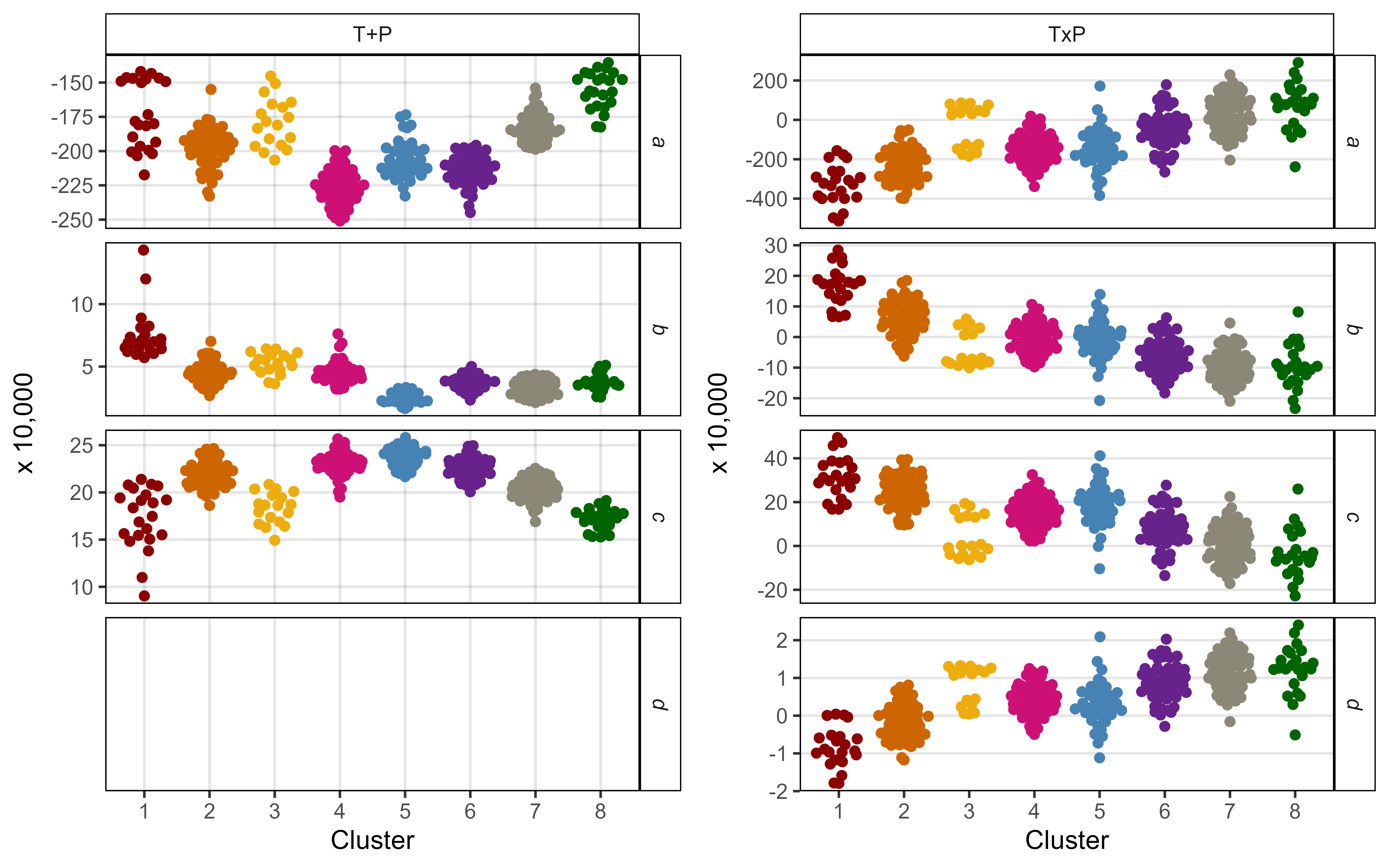
mp1 <- ggplot(xx %>% filter(Model=="T+P", !is.na(Value)),
aes(x = Cluster, y = Value * 10000, color = Cluster)) +
geom_quasirandom() +
theme_AGL +
theme(strip.text.y = element_text(face = "italic")) +
facet_grid(Coef ~ Model, scales = "free_y", drop = F) +
scale_color_manual(values = colors) + labs(y = "x 10,000")
mp2 <- ggplot(xx %>% filter(Model=="TxP"),
aes(x = Cluster, y = Value * 10000, color = Cluster)) +
geom_quasirandom() +
facet_grid(Coef ~ Model, scales = "free_y") +
theme_AGL +
theme(strip.text.y = element_text(face = "italic"),
panel.grid.major.x = element_blank()) +
scale_color_manual(values = colors) + labs(y = "x 10,000")
mp <- ggarrange(mp1, mp2, ncol = 2, legend = "none")
ggsave("Additional/Additional_Figure_11.png", mp, width = 8, height = 5, dpi = 600)Additional Figure 12: Coefficient p-values
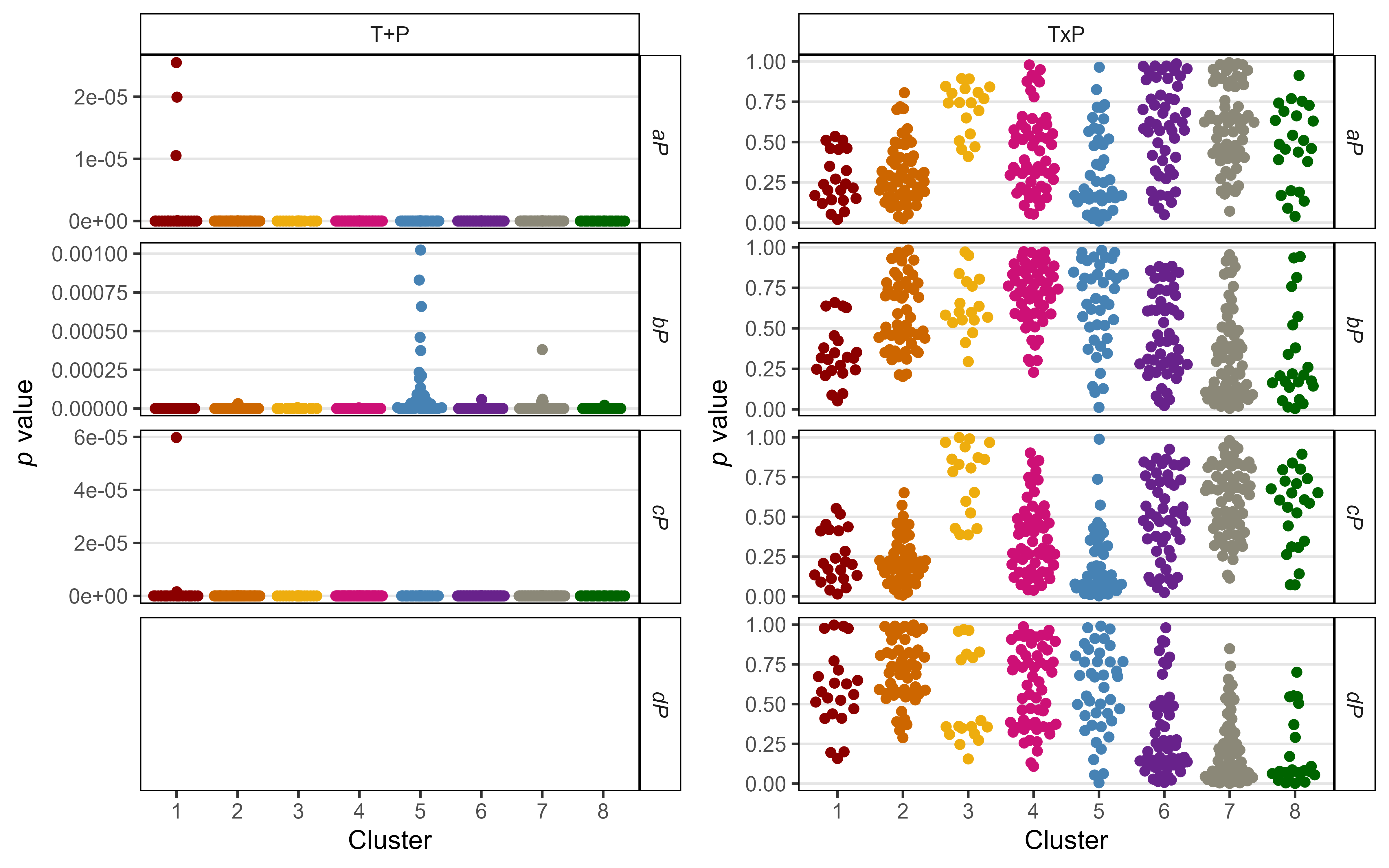
# Prep data
pca <- read.csv("data/data_pca_results.csv") %>% mutate(Cluster = factor(Cluster))
x1 <- read.csv("data/model_t+p_coefs.csv") %>% mutate(Model = "T+P")
x2 <- read.csv("data/model_txp_coefs.csv") %>% mutate(Model = "TxP")
xx <- bind_rows(x1, x2) %>%
  gather(Coef, Value, aP,bP,cP,dP) %>%
  left_join(pca, by = "Entry") %>%
  mutate(Cluster = factor(Cluster), Coef = factor(Coef))
# Plot
mp1 <- ggplot(xx %>% filter(Model=="T+P", !is.na(Value)),
              aes(x = Cluster, y = Value, color = Cluster)) +
  geom_quasirandom() +
  facet_grid(Coef ~ Model, scales = "free_y", drop = F) +
  scale_color_manual(values = colors) +
  theme_AGL +
  theme(strip.text.y = element_text(face = "italic"),
        panel.grid.major.x = element_blank())  +
  labs(y = expression(paste(italic("p"), " value")))
mp2 <- ggplot(xx%>%filter(Model=="TxP"),
              aes(x = Cluster, y = Value, color = Cluster)) +
  geom_quasirandom() +
  facet_grid(Coef ~ Model, scales = "free_y") +
  theme_AGL +
  theme(strip.text.y = element_text(face = "italic"),
        panel.grid.major.x = element_blank()) +
  scale_color_manual(values = colors) +
  labs(y = expression(paste(italic("p"), " value")))
mp <- ggarrange(mp1,mp2,ncol=2, legend = "none")
ggsave("Additional/Additional_Figure_12.png", mp, width = 8, height = 5, dpi = 600)
Additional Figure 13: p-values b c
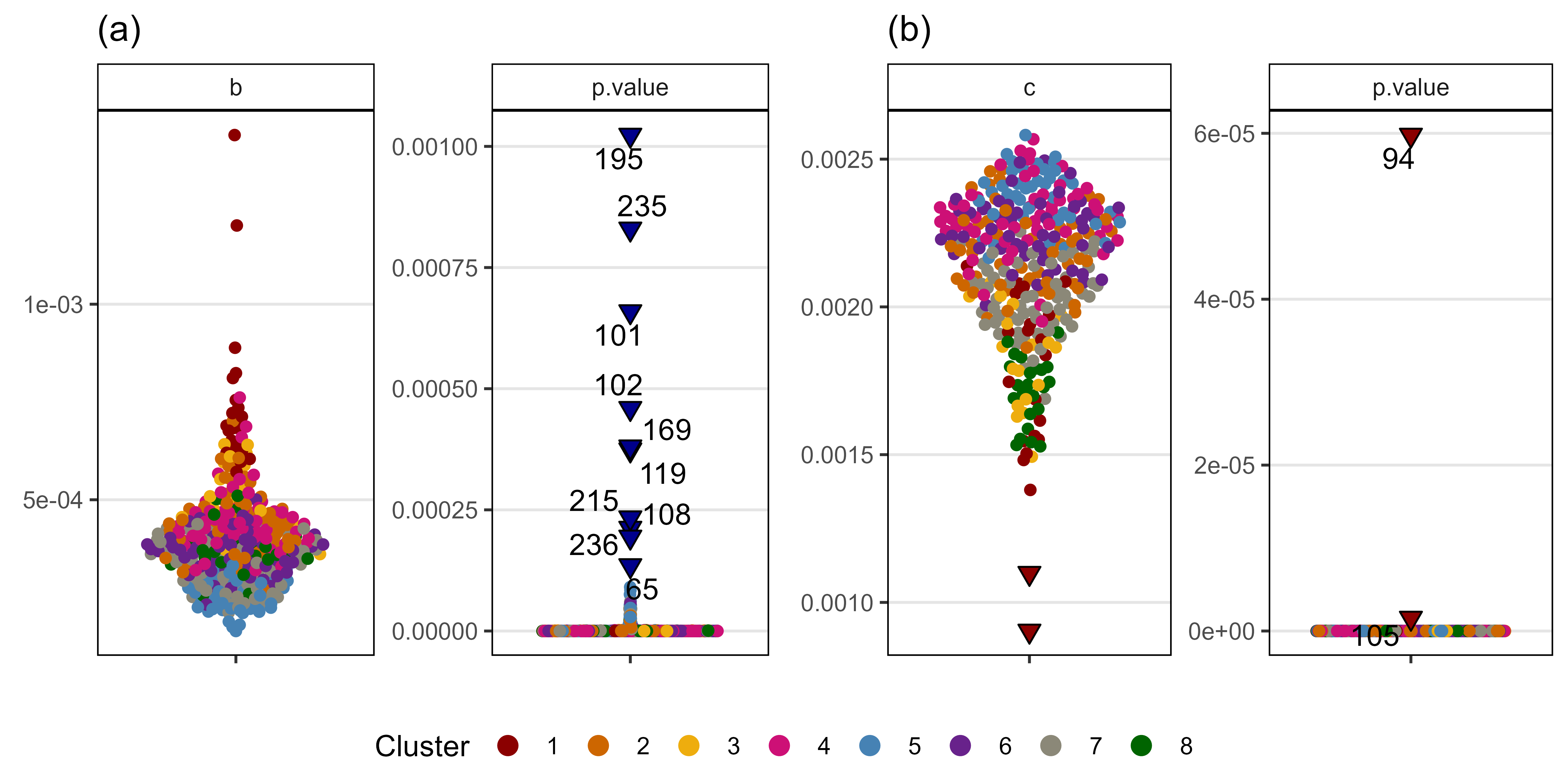
# Prep data
pca <- read.csv("data/data_pca_results.csv") %>%
  mutate(Cluster = factor(Cluster))
xx <- read.csv("data/model_t+p_coefs.csv") %>%
  mutate(Sig = factor(ifelse(bP > 0.0001, "Sig","Less Sig"))) %>%
  select(Entry, Sig, p.value=bP, b) %>%
  gather(Trait, Value, p.value, b) %>%
  left_join(pca, by = "Entry")
x1 <- xx %>% filter(Sig == "Sig", Trait == "p.value")
# Plot (a)
mp1 <- ggplot(xx, aes(x = "", y = Value, group = "")) +
  geom_quasirandom(aes(color = Cluster)) +
  geom_point(data = x1, size = 2.5, pch = 25,
             color = "black", fill = "darkblue") +
  geom_text_repel(data = x1, aes(label = Entry)) +
  facet_wrap(.~Trait, scales = "free_y") +
  scale_color_manual(values = colors) +
  guides(colour = guide_legend(nrow = 1, override.aes = list(size = 3))) +
  theme_AGL +
  theme(panel.grid.major.x = element_blank()) +
  labs(title = "(a)", x = NULL, y = NULL)
# Prep data
xx <- read.csv("data/model_t+p_coefs.csv") %>%
  mutate(Sig = factor(ifelse(cP > 0.000001, "Sig","Less Sig"))) %>%
  select(Entry, Sig, p.value=cP, c) %>%
  gather(Trait, Value, p.value, c) %>%
  left_join(pca, by = "Entry")
x1 <- xx %>% filter(Sig == "Sig")
# Plot B)
mp2 <- ggplot(xx, aes(x = "", y = Value, group = "")) +
  geom_quasirandom(aes(color = Cluster)) +
  geom_point(data = x1, size = 2.5, pch = 25,
             color = "black", fill = "darkred") +
  geom_text_repel(data = x1 %>% filter(Trait =="p.value"), aes(label = Entry)) +
  facet_wrap(.~Trait, scales = "free_y") +
  scale_color_manual(values = colors) +
  guides(colour = guide_legend(nrow = 1, override.aes = list(size = 3))) +
  theme_AGL +
  theme(panel.grid.major.x = element_blank()) +
  labs(title = "(b)", x = NULL, y = NULL)
# Append (a) and (b)
mp <- ggarrange(mp1, mp2, ncol = 2, common.legend = T, legend = "bottom")
ggsave("Additional/Additional_Figure_13.png", mp, width = 8, height = 4, dpi = 600, bg = "white")
Modeling DTF (T + P) - Location Out
Train the model without the location used for prediction
####################################
# 1/f = a + bT + cP (Location Out) #
####################################
# Prep data
xx <- rr %>%
  filter(!is.na(RDTF)) %>%
  left_join(select(ff, Expt, T_mean, P_mean), by = "Expt")
mr <- NULL
md <- NULL
# Model - For each Location, the model is re-trained without that locations data
for(i in 1:324) {
  for(k in unique(xx$Location)) {
    # Prep data
    xi1 <- xx %>% filter(Entry == i, Location != k)
    xi2 <- xx %>% filter(Entry == i, Location == k)
    xd2 <- xi2 %>%
      group_by(Entry, Name, Expt, ExptShort) %>%
      summarise_at(vars(DTF, RDTF, T_mean, P_mean), funs(mean), na.rm = T) %>%
      ungroup()
    # Train model
    mi <- lm(RDTF ~ T_mean * P_mean, data = xi1)
    # Predict DTF
    xi2 <- xi2 %>% mutate(Predicted_DTF = 1 / predict(mi, newdata = xi2))
    xd2 <- xd2 %>% mutate(Predicted_DTF = 1 / predict(mi, newdata = xd2))
    # Save to table
    mr <- bind_rows(mr, xi2)
    md <- bind_rows(md, xd2)
  }
}
# Save Results
write.csv(mr, "data/model_test.csv", row.names = F)
write.csv(md, "data/model_test_d.csv", row.names = F)
Figure 4: Test Model
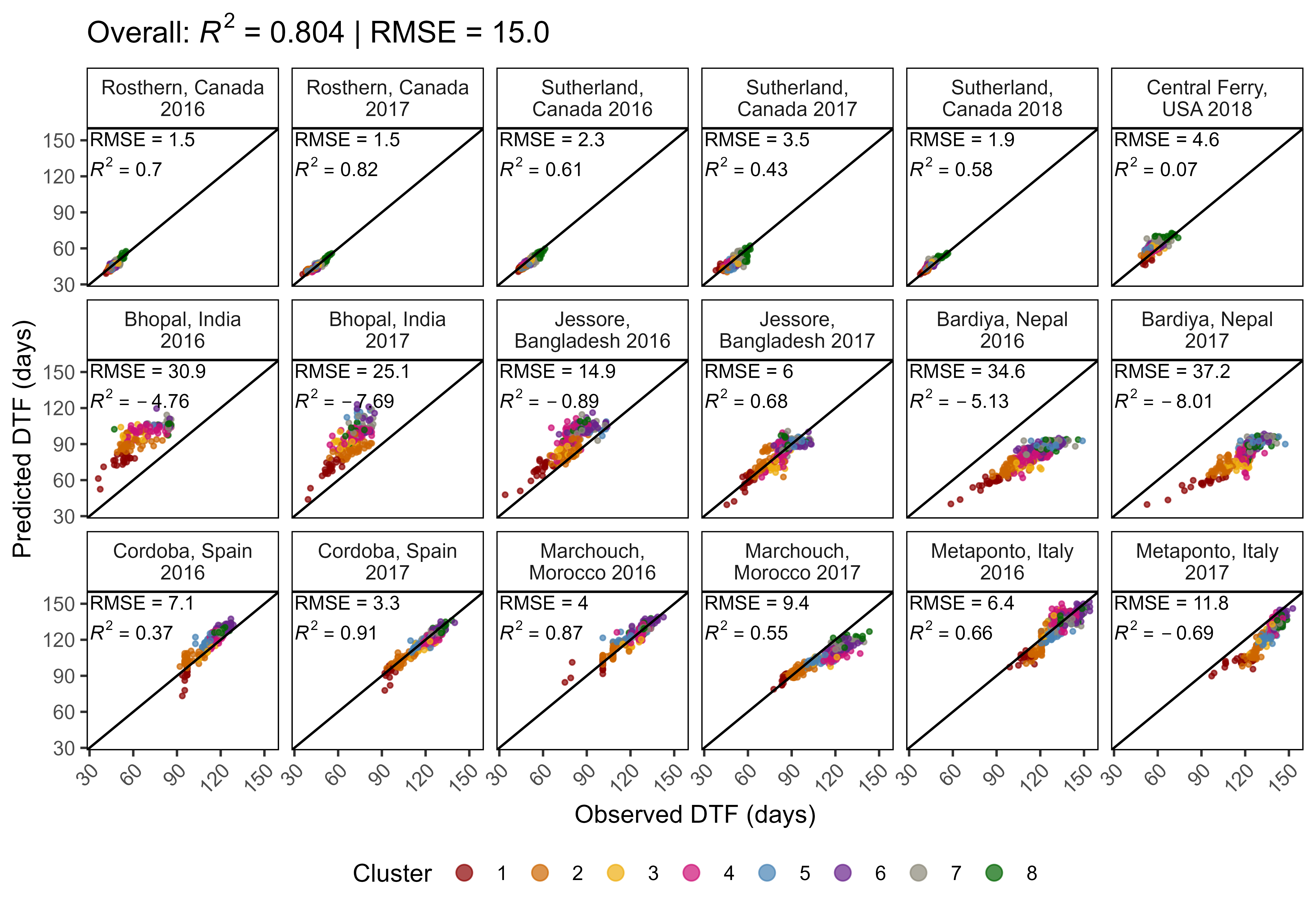
Figure 4: Comparison of observed and predicted values for days from sowing to flowering (DTF) for a lentil (Lens culinaris Medik.) diversity panel calculated using equation 1. For each site-year, the model was retrained after removing all observations from that location, regardless of year before predicting results from that location. R2 = coefficient of determination, RMSE = root-mean-square error.
# Prep data
xx <- read.csv("data/model_test_d.csv") %>%
  mutate(Expt = factor(Expt, levels = names_Expt))
# Plot Observed vs Predicted
mp <- ggModel2(xx, title = expression(paste("Overall: ", italic("R")^2, " = 0.804 | RMSE = 15.0")))
ggsave("Figure_04.png", mp, width = 8, height = 5.5, dpi = 600)[1] 0.8045254[1] 15.01078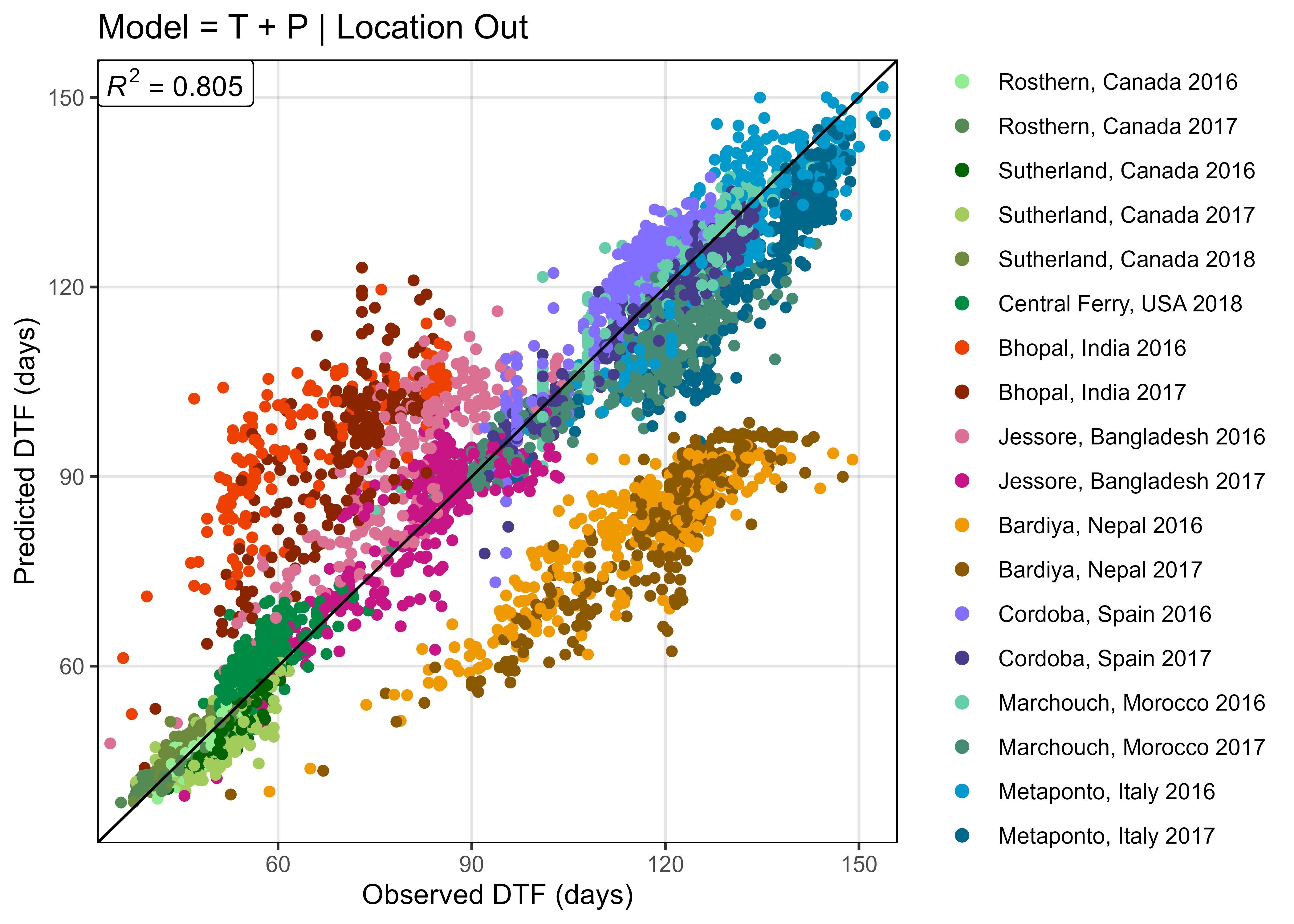
# Plot Observed vs Predicted
mp <- ggModel1(xx, title = "Model = T + P | Location Out")
ggsave("Additional/Model/Model_1_3.png", mp, width = 7, height = 5, dpi = 600)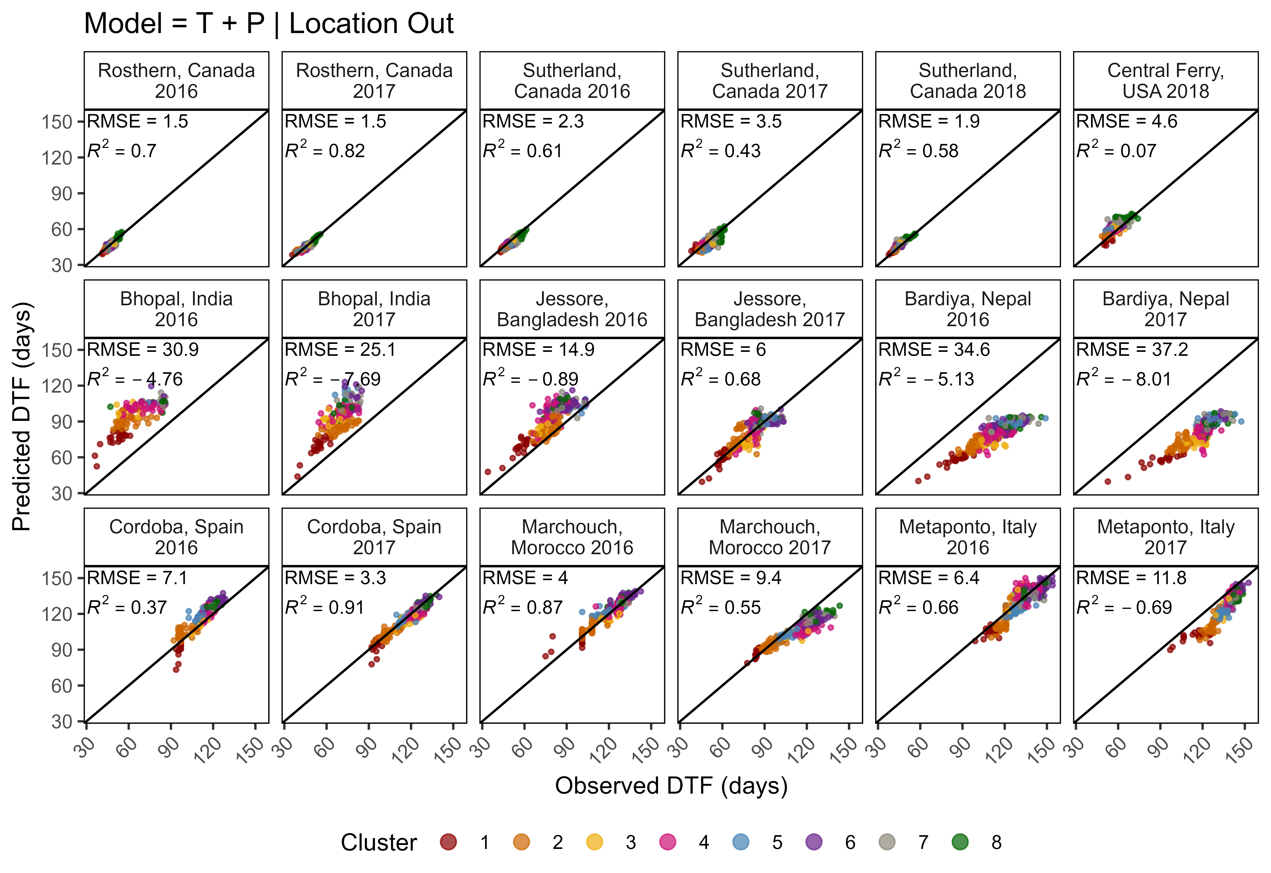
# Plot Observed vs Predicted
mp <- ggModel2(xx, title = "Model = T + P | Location Out")
ggsave("Additional/Model/Model_2_3.png", mp, width = 8, height = 5.5, dpi = 600)
Supplemental Table 4: Test Model
Table S4: All possible combinations of a single temperate, South Asian, and Mediterranean site-year, used to train the model, with equation 1, along with the corresponding coefficient of determination (RR = R2), and number of genotypes which flowered in all three site-years.
####################################
# 1/f = a + bT + cP (3 Locations) #
####################################
# Prep data
xx <- rr %>% #filter(!is.na(DTF)) %>%
  left_join(select(ff, Expt, T_mean, P_mean), by = "Expt")
mt <- data.frame(Temperate_Location  = rep(names_ExptShort[1:6],  each = 36),
                 SouthAsian_Location = rep(names_ExptShort[7:12], times = 36)) %>%
  arrange(SouthAsian_Location) %>%
  mutate(Mediterranean_Location = rep(names_ExptShort[13:18], 36),
                 RR = NA, Genotypes = NA)
# Run each combination
for(t in names_ExptShort[1:6]) { # Temperate site-years
  for(s in names_ExptShort[7:12]) { # South asian site-years
    for(m in names_ExptShort[13:18]) { # Mediterranean site-years
      mr <- NULL; md <- NULL
      for(i in 1:324) {
        # Prep data
        xi1 <- xx %>% filter(Entry == i, ExptShort %in% c(t, s, m))
        xi2 <- xx %>% filter(Entry == i)
        xd2 <- xi2 %>%
          group_by(Entry, Name, Expt, ExptShort) %>%
          summarise_at(vars(DTF, RDTF, T_mean, P_mean), funs(mean), na.rm = T) %>%
          ungroup()
        # Train model
        mi <- lm(RDTF ~ T_mean + P_mean, data = xi1)
        # Predict DTF
        xi2 <- xi2 %>% mutate(Predicted_DTF = 1 / predict(mi, newdata = xi2))
        xd2 <- xd2 %>% mutate(Predicted_DTF = 1 / predict(mi, newdata = xd2))
        # Save to table
        mr <- bind_rows(mr, xi2)
        md <- bind_rows(md, xd2)
      }
      remEntries <- unique(md$Entry[is.na(md$DTF) & md$ExptShort %in% c(t, s, m)])
      md2 <- md %>% filter(!Entry %in% remEntries, !md$ExptShort %in% c(t, s, m))
      myrow <- mt$Temperate_Location     == t &
               mt$SouthAsian_Location    == s &
               mt$Mediterranean_Location == m
      mt[myrow,"RR"] <- round(modelR2(md2$DTF, md2$Predicted_DTF), 6)
      mt[myrow,"Genotypes"] <- length(unique(md2$Entry))
    }
  }
}
# Save
write.csv(mt %>% arrange(RR), "Supplemental_Table_04.csv", row.names = F)
Modeling DTF (T + P) - 3 Best
####################################
# 1/f = a + bT + cP (3 Locations) #
####################################
# Prep data
xx <- rr %>%
  filter(!is.na(RDTF)) %>%
  left_join(select(ff, Expt, T_mean, P_mean), by = "Expt")
mr <- NULL
md <- NULL
mc <- select(ldp, Entry, Name) %>%
  mutate(a = NA, b = NA, c = NA, RR = NA, Environments = NA )
k <- c("Sutherland, Canada 2016", "Jessore, Bangladesh 2017", "Cordoba, Spain 2017")
# Model - only the ^above^ three site-years are used to train the model
for(i in 1:324) {
  # Prep data
  xi1 <- xx %>% filter(Entry == i, Expt %in% k)
  xi2 <- xx %>% filter(Entry == i)
  xd2 <- xi2 %>%
    group_by(Entry, Name, Expt, ExptShort) %>%
    summarise_at(vars(DTF, RDTF, T_mean, P_mean), funs(mean), na.rm = T) %>%
    ungroup()
  # Train model
  mi <- lm(RDTF ~ T_mean * P_mean, data = xi1)
  # Predict DTF
  xi2 <- xi2 %>% mutate(Predicted_DTF = 1 / predict(mi, newdata = xi2))
  xd2 <- xd2 %>% mutate(Predicted_DTF = 1 / predict(mi, newdata = xd2))
  # Save to table
  mr <- bind_rows(mr, xi2)
  md <- bind_rows(md, xd2)
  # Save coefficients
  mc[i,c(3:5)] <- mi$coefficients
  # Calculate rr and # of environments used
  mc[i,6] <- 1 - sum((xi2$DTF - xi2$Predicted_DTF)^2) / sum((xi2$Predicted_DTF - mean(xi2$DTF))^2)
  mc[i,7] <- length(unique(xi2$Expt))
}
ents <- xx %>% filter(ExptShort %in% c("Su16", "Ba17", "Sp17"), is.na(DTF)) %>%
  pull(Entry) %>% unique()
mr <- mr %>% filter(!Entry %in% ents)
md <- md %>% filter(!Entry %in% ents)
mc <- mc %>% filter(!Entry %in% ents)
# Save Results
write.csv(mr, "data/model_3best.csv",        row.names = F)
write.csv(md, "data/model_3best_d.csv",      row.names = F)
write.csv(mc, "data/model_3best_coefs.csv",  row.names = F)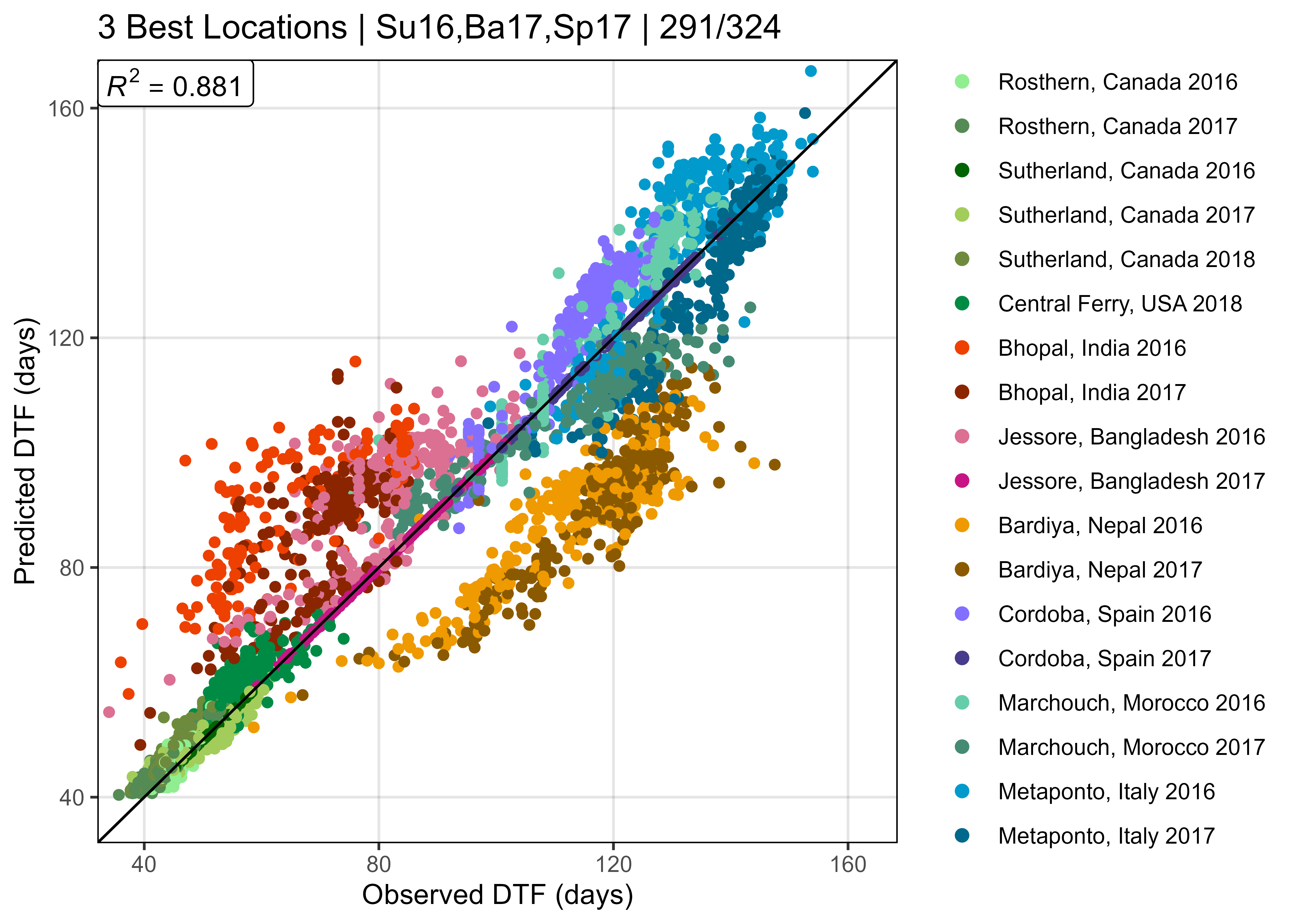
# Prep data
xx <- read.csv("data/model_3best_d.csv") %>%
  mutate(Expt = factor(Expt, levels = names_Expt))
# Plot Observed vs Predicted
mp <- ggModel1(xx, title = "3 Best Locations | Su16,Ba17,Sp17 | 291/324")
ggsave("Additional/Model/Model_1_4.png", mp, width = 7, height = 5, dpi = 600)
#
length(unique(xx$Entry))
[1] 291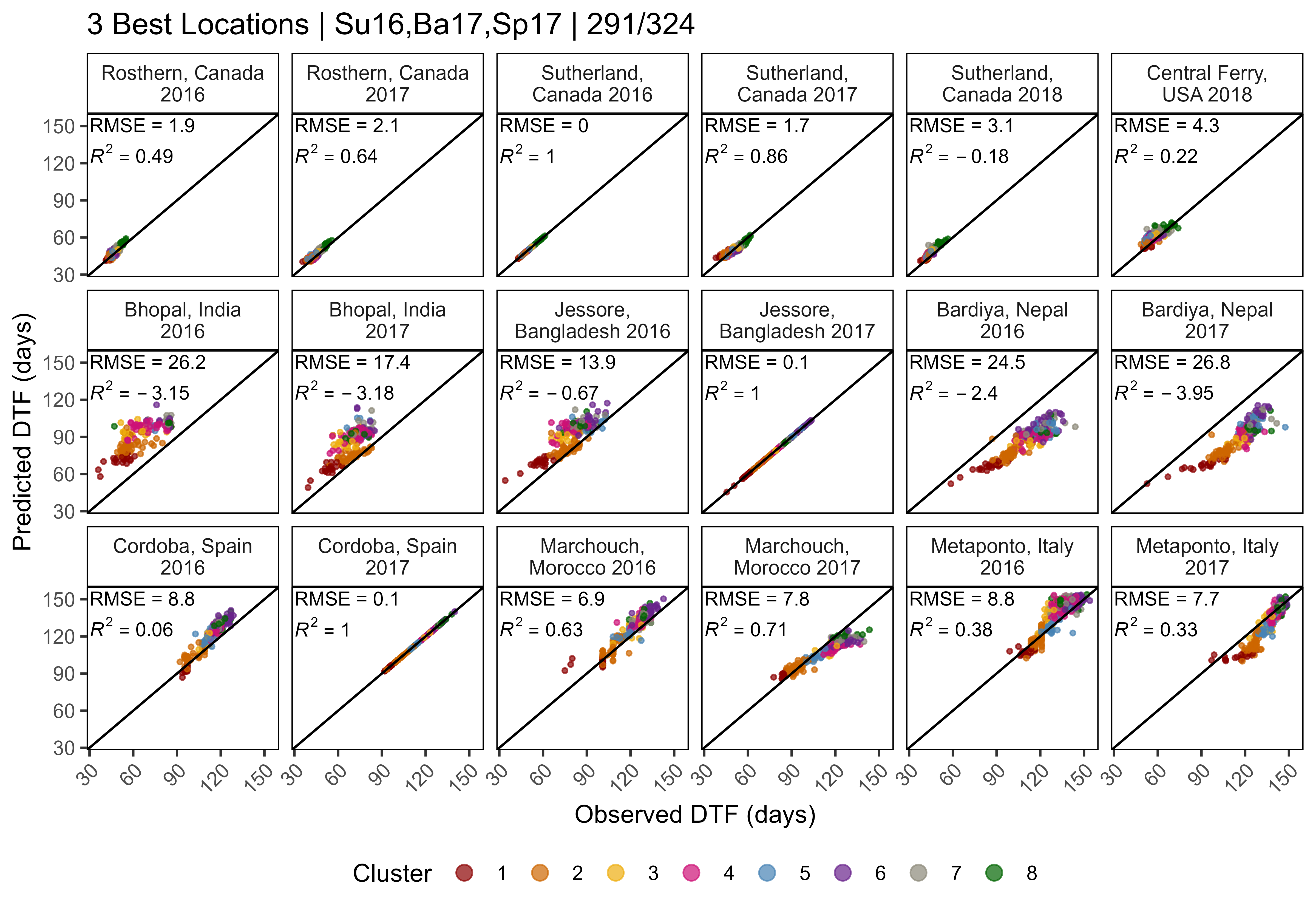
# Plot B)
mp <- ggModel2(xx, title = "3 Best Locations | Su16,Ba17,Sp17 | 291/324")
ggsave("Additional/Model/Model_2_4.png", mp, width = 8, height = 5.5, dpi = 600)
Modeling DTF (T + P) - 3 Worst
####################################
# 1/f = a + bT + cP (3 Locations)  #
####################################
# Prep data
xx <- rr %>%
  filter(!is.na(RDTF)) %>%
  left_join(select(ff, Expt, T_mean, P_mean), by = "Expt")
mr <- NULL
md <- NULL
mc <- select(ldp, Entry, Name) %>%
  mutate(a = NA, b = NA, c = NA, RR = NA, Environments = NA )
k <- c("Sutherland, Canada 2018", "Bhopal, India 2016", "Cordoba, Spain 2016")
# Model - only the ^above^ three site-years are used to train the model
for(i in 1:324) {
  # Prep data
  xi1 <- xx %>% filter(Entry == i, Expt %in% k)
  xi2 <- xx %>% filter(Entry == i)
  xd2 <- xi2 %>%
    group_by(Entry, Name, Expt, ExptShort) %>%
    summarise_at(vars(DTF, RDTF, T_mean, P_mean), funs(mean), na.rm = T) %>%
    ungroup()
  # Train model
  mi <- lm(RDTF ~ T_mean * P_mean, data = xi1)
  # Predict DTF
  xi2 <- xi2 %>% mutate(Predicted_DTF = 1 / predict(mi, newdata = xi2))
  xd2 <- xd2 %>% mutate(Predicted_DTF = 1 / predict(mi, newdata = xd2))
  # Save to table
  mr <- bind_rows(mr, xi2)
  md <- bind_rows(md, xd2)
  # Save coefficients
  mc[i,c(3:5)] <- mi$coefficients
  # Calculate rr and # of environments used
  mc[i,6] <- 1 - sum((xi2$DTF - xi2$Predicted_DTF)^2) /
    sum((xi2$Predicted_DTF - mean(xi2$DTF))^2)
  mc[i,7] <- length(unique(xi2$Expt))
}
ents <- xx %>%
  filter(ExptShort %in% c("Su18", "In16", "Sp16"), is.na(DTF)) %>%
  pull(Entry) %>% unique()
mr <- mr %>% filter(!Entry %in% ents)
md <- md %>% filter(!Entry %in% ents)
mc <- mc %>% filter(!Entry %in% ents)
# Save Results
write.csv(mr, "data/model_3worst.csv",        row.names = F)
write.csv(md, "data/model_3worst_d.csv",      row.names = F)
write.csv(mc, "data/model_3worst_coefs.csv",  row.names = F)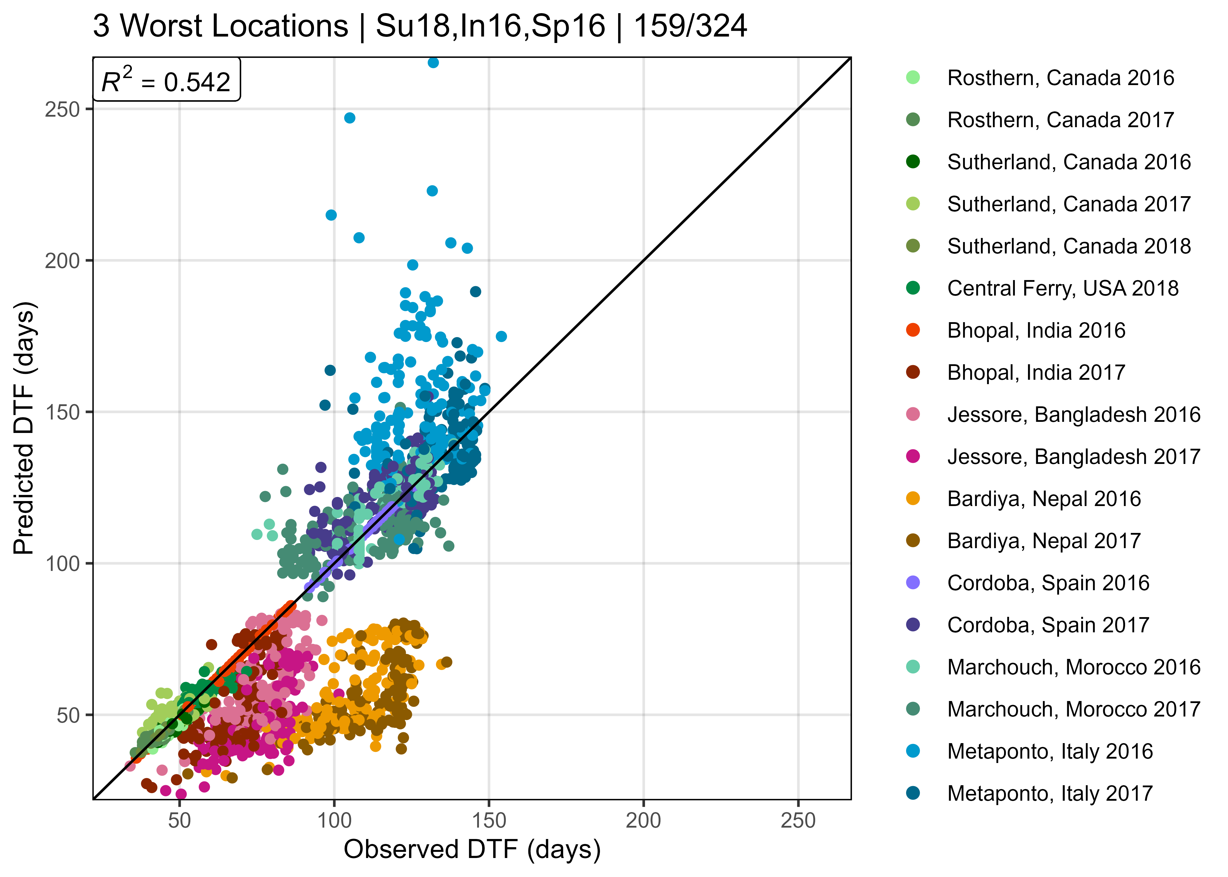
# Prep data
xx <- read.csv("data/model_3worst_d.csv") %>%
  mutate(Expt = factor(Expt, levels = names_Expt))
# Plot Observed vs Predicted
mp <- ggModel1(xx, title = "3 Worst Locations | Su18,In16,Sp16 | 159/324")
ggsave("Additional/Model/Model_1_5.png", mp, width = 7, height = 5, dpi = 600)
#
length(unique(xx$Entry))
[1] 159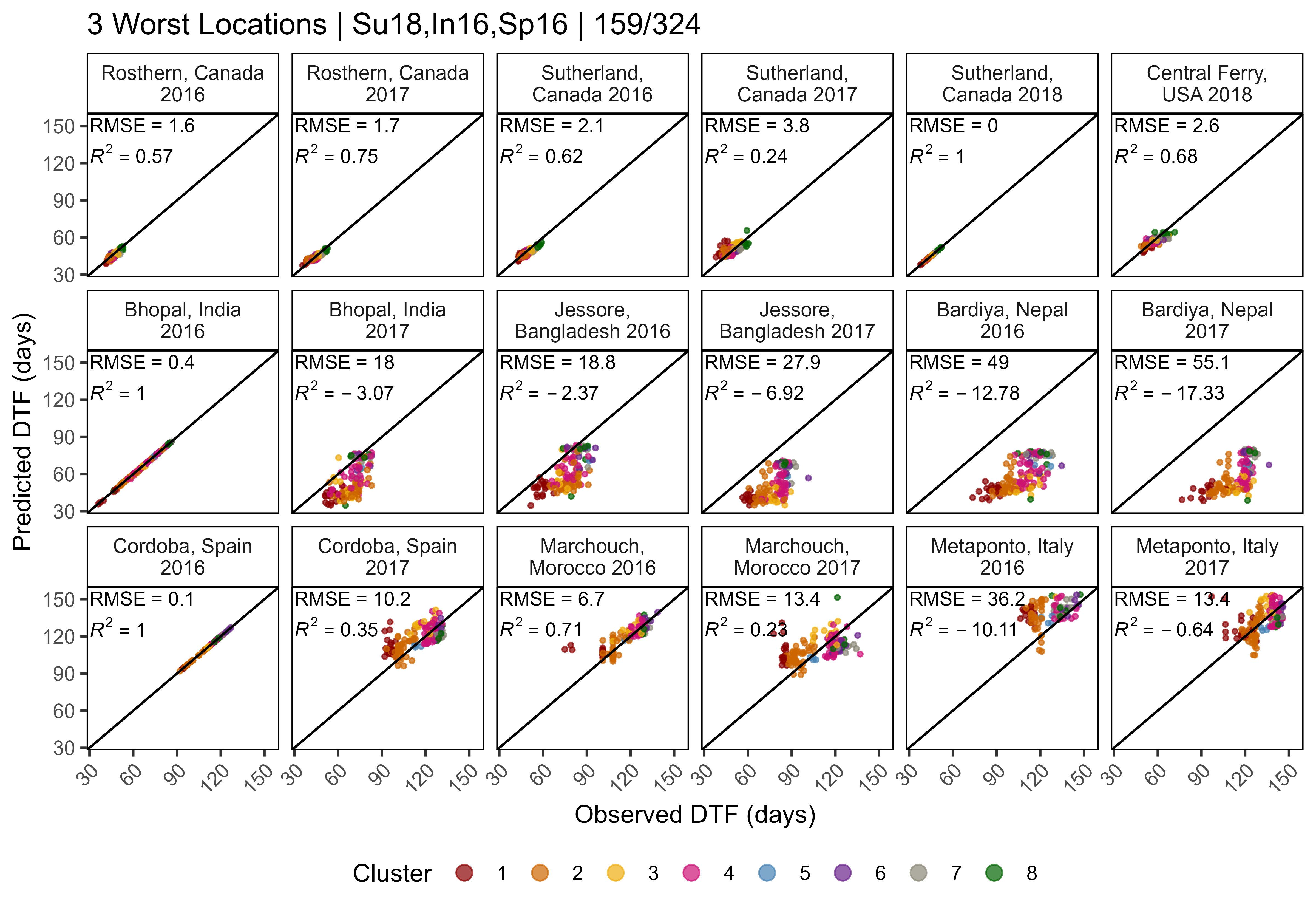
# Plot B)
mp <- ggModel2(xx, title = "3 Worst Locations | Su18,In16,Sp16 | 159/324")
ggsave("Additional/Model/Model_2_5.png", mp, width = 8, height = 5.5, dpi = 600)
DTF Model Correlation Coefficients
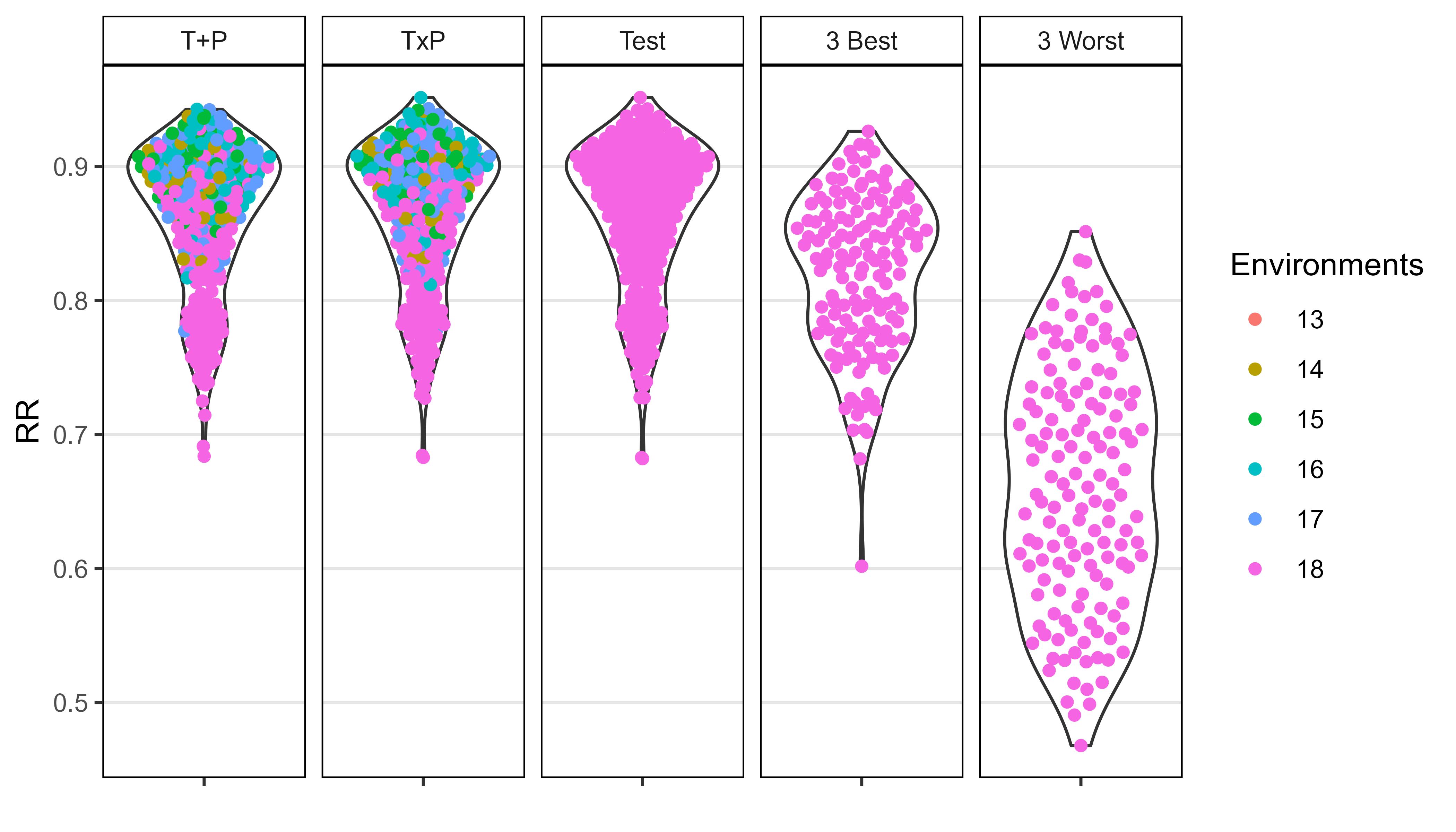
# Prep data
x1 <- read.csv("data/model_t+p_coefs.csv") %>% mutate(Model = "T+P")
x2 <- read.csv("data/model_txp_coefs.csv") %>% mutate(Model = "TxP")
x3 <- read.csv("data/model_test_coefs.csv") %>% mutate(Model = "Test")
x4 <- read.csv("data/model_3best_coefs.csv")  %>% mutate(Model = "3 Best")
x5 <- read.csv("data/model_3worst_coefs.csv")  %>% mutate(Model = "3 Worst")
xx <- bind_rows(x1, x2, x3, x4, x5) %>%
  mutate(Model = factor(Model, levels = unique(Model)),
         Environments = factor(Environments))
# Plot RR
mp <- ggplot(xx, aes(x = "", y = RR)) +
  geom_violin() +
  geom_quasirandom(aes(color = Environments)) +
  facet_grid(. ~ Model) +
  theme_AGL +
  theme(panel.grid.major.x = element_blank()) +
  labs(x = NULL)
ggsave("Additional/Model/Model_pvalues.png", mp, width = 7, height = 4, dpi = 600)
Supplemental Figure 6: Compare Constants Entry
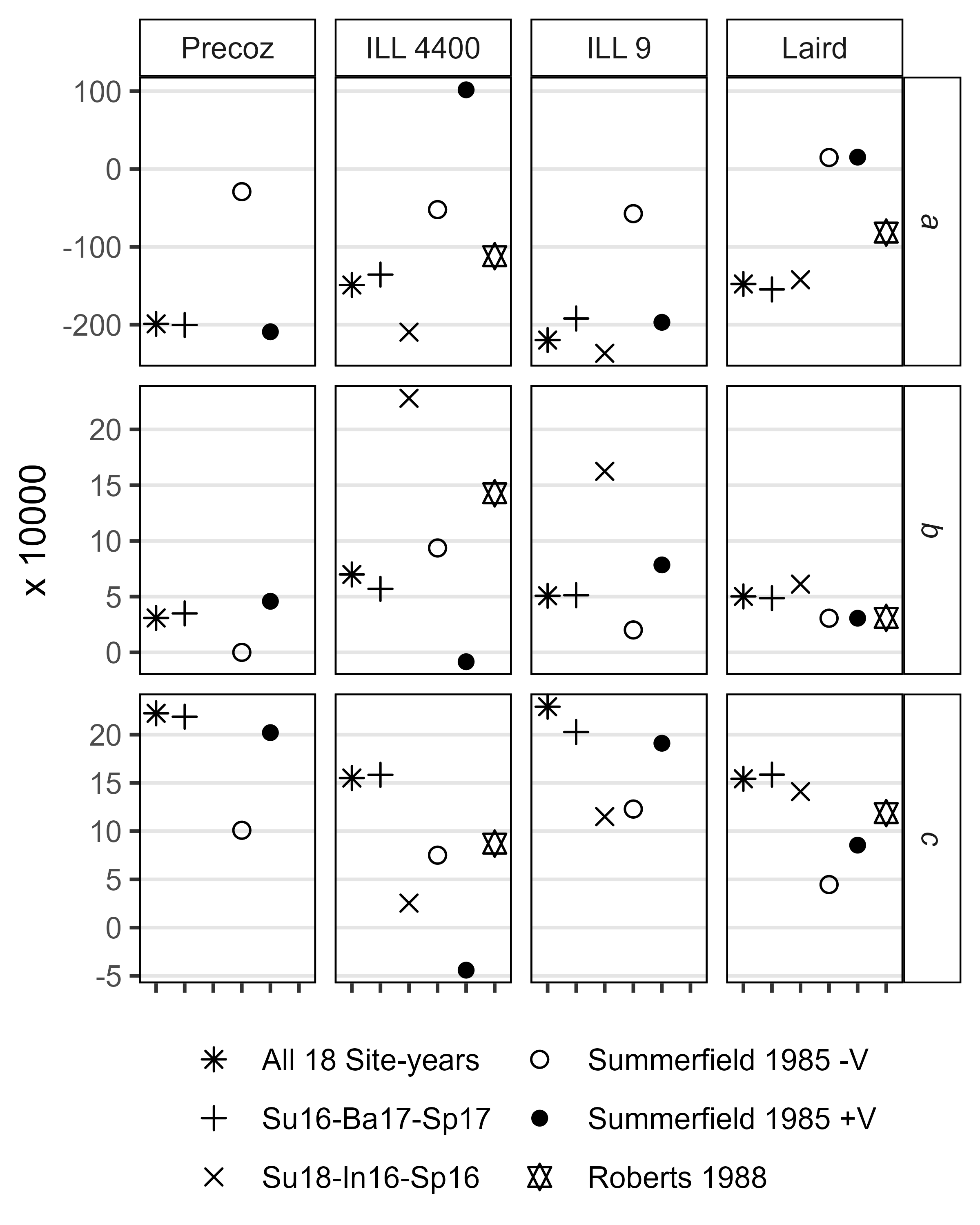
Figure S6: Comparison of a, b, and c constants calculated using equation 1, in the current study using all site-years, the three best site-years for predicting DTF, Sutherland, Canada 2016 (Su16), Jessore, Bangladesh 2017 (Ba17) and Cordoba, Spain 2017 (Sp17), the three worst site-years for predicting DTF, Sutherland, Canada 2018 (Su18), Bhopal, India 2016 (In16) and Cordoba, Spain 2016 (Sp16), from Roberts et al., (1988) and from Summerfield et al., (1985) with (+V) and without (-V) a seed vernalization treatment.
- Entry 76 = ILL 4400 (Syrian Local Large)
- Entry 77 = ILL 4605 (Precoz)
- Entry 118 = ILL 9
- Entry 128 = Laird
# Prep data
x1 <- read.csv("data/model_t+p_coefs.csv") %>%
  filter(Entry %in% c(76, 77, 118, 128)) %>%
  mutate(Expt = "All 18 Site-years")
x2.1 <- read.csv("data/model_3best_coefs.csv") %>%
  filter(Entry %in% c(76, 77, 118, 128)) %>%
  mutate(Expt = "Su16-Ba17-Sp17")
x2.2 <- read.csv("data/model_3worst_coefs.csv") %>%
  filter(Entry %in% c(76, 77, 118, 128)) %>%
  mutate(Expt = "Su18-In16-Sp16")
# Summerfield et al., 1985
x3 <- x1 %>% mutate(Expt = "Summerfield 1985 -V")
x3[x3$Entry == 76,  c("a","b","c")] <- c(-0.002918,  0,          0.0010093)
x3[x3$Entry == 77,  c("a","b","c")] <- c(-0.0052226, 0.00093643, 0.00075104)
x3[x3$Entry == 118, c("a","b","c")] <- c(-0.0057408, 0.00020113, 0.0012292)
x3[x3$Entry == 128, c("a","b","c")] <- c( 0.0014689, 0.00030622, 0.00044640)
x4 <- x1 %>% mutate(Expt = "Summerfield 1985 +V")
x4[x4$Entry == 76,  c("a","b","c")] <- c(-0.020910,   0.00045813,  0.0020210)
x4[x4$Entry == 77,  c("a","b","c")] <- c( 0.0101590, -0.00008401, -0.00044067)
x4[x4$Entry == 118, c("a","b","c")] <- c(-0.0196948,  0.00078441,  0.0019110)
x4[x4$Entry == 128, c("a","b","c")] <- c( 0.0015094,  0.00030622,  0.00085502)
# Roberts et al., 1988
x5 <- x1 %>% filter(Entry %in% c(77, 128)) %>% mutate(Expt = "Roberts 1988")
x5[x5$Entry == 77,  c("a","b","c")] <- c(-0.0112,   0.001427, 0.000871)
x5[x5$Entry == 128, c("a","b","c")] <- c(-0.008172, 0.000309, 0.001187)
#
xx <- bind_rows(x1, x2.1, x2.2, x3, x4, x5) %>%
  gather(Constant, Value, a, b, c) %>%
  mutate(Entry = factor(Entry),
         Name = plyr::mapvalues(Entry, c(76,77,118,128),
                  c("Precoz","ILL 4400","ILL 9","Laird")),
         Expt = factor(Expt, levels = c("All 18 Site-years",
                  "Su16-Ba17-Sp17", "Su18-In16-Sp16",
                  "Summerfield 1985 -V", "Summerfield 1985 +V", "Roberts 1988")))
# Plot
mp <- ggplot(xx, aes(x = Expt, y = Value * 10000, shape = Expt)) +
  geom_quasirandom(size = 2, width = 0.2) +
  facet_grid(Constant ~ Name, scales = "free_y") +
  scale_shape_manual(name = NULL, values = c(8,3,4,1,16,11)) +
  guides(shape=guide_legend(nrow = 3, byrow = F)) +
  theme_AGL +
  theme(legend.position = "bottom", legend.margin = unit(c(0,0,0,0), "cm"),
        strip.text.y = element_text(face = "italic"),
        panel.grid.major.x = element_blank(),
        axis.text.x = element_blank()) +
  labs(x = NULL, y = "x 10000")
ggsave("Supplemental_Figure_06.png", mp, width = 4, height = 5, dpi = 600)
Supplemental Figure 7: 3 best vs. 3 worst
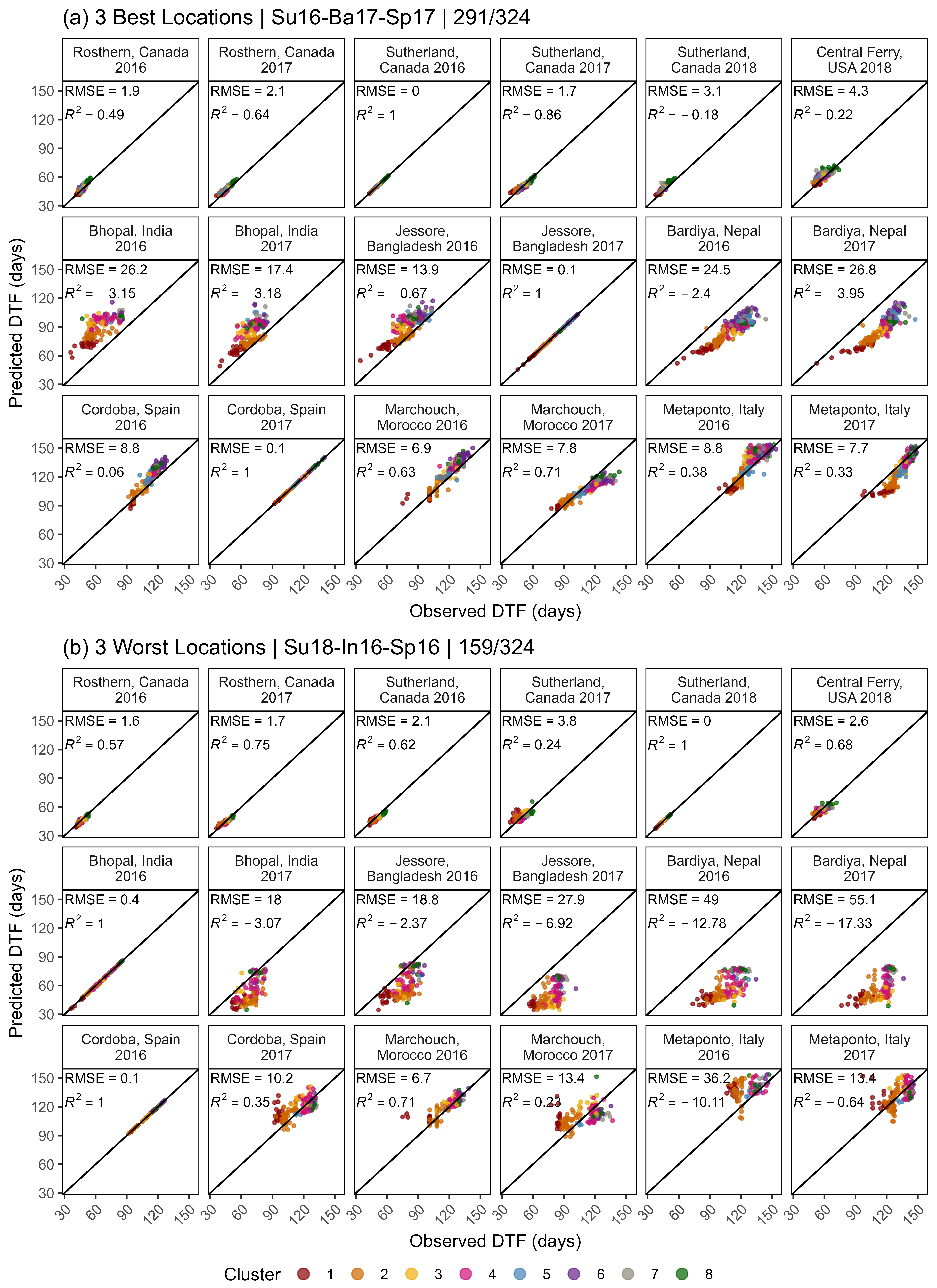
Figure S7: Comparison of observed and predicted values, along with the coefficient of determination (R2) and root-mean-square error (RMSE), for days from sowing to flowering, calculated using equation 1, with (a) the 3 best site-years for training the model and (b) the 3 worst years for training the model (see Table S4). Sutherland, Canada 2016 and 2018 (Su16, Su18), Cordoba, Spain 2016 and 2017 (Sp16, Sp17), Bhopal, India 2016 (In16) and Jessore, Bangladesh 2017 (Ba17). Predictions of DTF can only be made with genotypes that flowered in all three locations, therefore, predictions in (a) are based on 291 and in (b) based on 159 of 324 genotypes used in this study.
# Plot (a)
xx <- read.csv("data/model_3best_d.csv") %>%
  mutate(Expt = factor(Expt, levels = names_Expt))
mp1 <- ggModel2(xx, title = "(a) 3 Best Locations | Su16-Ba17-Sp17 | 291/324")
# Plot (b)
xx <- read.csv("data/model_3worst_d.csv") %>%
  mutate(Expt = factor(Expt, levels = names_Expt))
mp2 <- ggModel2(xx, title = "(b) 3 Worst Locations | Su18-In16-Sp16 | 159/324")
# Append (a) and (b)
mp <- ggarrange(mp1, mp2, ncol = 1, common.legend = T, legend = "bottom")
ggsave("Supplemental_Figure_07.png", mp, width = 8, height = 11, dpi = 600, bg = "white")
Supplemental Figure 8: Compare Constants All
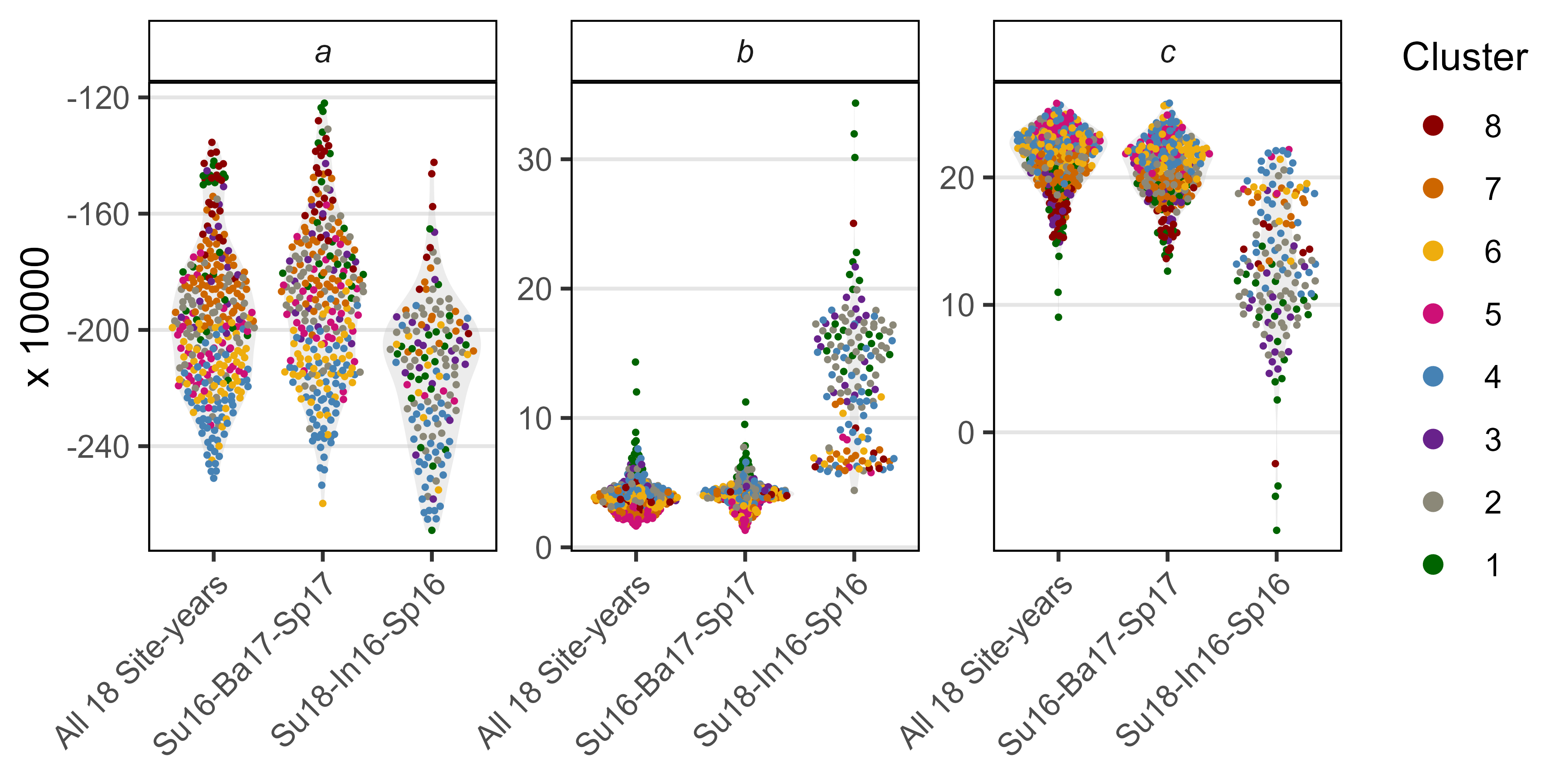
Figure S8: Comparison of a, b, and c constants calculated using equation 1 using all site-years, the three best site-years for predicting DTF, Sutherland, Canada 2016 (Su16), Jessore, Bangladesh 2017 (Ba17) and Cordoba, Spain 2017 (Sp17), and the three worst site-years for predicting DTF, Sutherland, Canada 2018 (Su18), Bhopal, India 2016 (In16) and Cordoba, Spain 2016 (Sp16).
# Prep data
levs <- c("All 18 Site-years", "Su16-Ba17-Sp17", "Su18-In16-Sp16")
pca <- read.csv("data/data_pca_results.csv") %>%
  select(Entry, Cluster) %>%
  mutate(Cluster = factor(Cluster))
x1 <- read.csv("data/model_t+p_coefs.csv") %>%
  mutate(Expt = levs[1]) %>% select(-RR)
x2 <- read.csv("data/model_3best_coefs.csv") %>%
  mutate(Expt = levs[2])
x3 <- read.csv("data/model_3worst_coefs.csv") %>%
  mutate(Expt = levs[3])
xx <- bind_rows(x1, x2,x3) %>%
  left_join(pca, by = "Entry") %>%
  gather(Trait, Value, a, b, c) %>%
  mutate(Expt = factor(Expt,levels = levs))
# Plot
mp <- ggplot(xx, aes(x = Expt, y = Value * 10000, group = Expt)) +
  geom_violin(alpha = 0.3, color = NA, fill = "grey") +
  geom_quasirandom(aes(color = Cluster), size = 0.3) +
  facet_wrap(Trait ~ ., scales = "free") +
  scale_color_manual(values = colors, breaks = 8:1) +
  theme_AGL +
  theme(strip.text = element_text(face = "italic"),
        panel.grid.major.x = element_blank(),
        axis.text.x = element_text(angle = 45, hjust = 1)) +
  guides(colour = guide_legend(override.aes = list(size = 2))) +
  labs(x = NULL, y = "x 10000")
ggsave("Supplemental_Figure_08.png", mp, width = 6, height = 3, dpi = 600)
Base Temperature & Critical Photoperiod
# Calculate Tf and Pf
xx <- read.csv("data/model_t+p_coefs.csv") %>% select(-Name) %>%
  mutate(predicted_Tf = 1/b, predicted_Pf = 1/c )
xx <- rr %>% left_join(xx, by = "Entry") %>%
  left_join(select(ff, Expt, T_mean, P_mean), by = "Expt") %>%
  mutate(Tb = -(a + c * P_mean) / b,
         Pc = -(a + b * T_mean) / c,
         Tf_0 = NA, Tf_5 = NA, Tf = NA, Pf = NA, PTT = NA)
for(i in 1:nrow(xx)) {
  e1 <- ee %>% filter(Expt == xx$Expt[i])
  for(k in 1:nrow(e1)) {
    e1$Tfsum[k] <- sum(e1$Temp_mean[1:k] - xx$Tb[i])
    e1$Pfsum[k] <- sum(e1$DayLength[1:k] - xx$Pc[i])
  }
  ei <- e1 %>%
    filter(Date <= xx$PlantingDate[i] + xx$DTF2[i], !is.na(Temp_mean))
  if(nrow(ei) > 0) {
    xx$Tf_0[i]  <- round(sum(ei$Temp_mean), 1)
    xx$Tf_5[i]  <- round(sum(ei$Temp_mean - 5), 1)
    xx$Tf[i]    <- round(sum(ei$Temp_mean - xx$Tb[i]), 1)
    xx$Pf_0[i]  <- round(sum(ei$DayLength), 1)
    xx$Pf_7[i]  <- round(sum(ei$DayLength - 7), 1)
    xx$Pf[i]    <- round(sum(ei$DayLength - xx$Pc[i]), 1)
    xx$PTT_0[i] <- round(sum(ei$Temp_mean * ei$DayLength), 1)
    xx$PTT[i]   <- round(sum((ei$Temp_mean - xx$Tb[i]) * (ei$DayLength - xx$Pc[i])), 1)
    eTf <- e1 %>% filter(Tfsum > xx$predicted_Tf[i])
    ePf <- e1 %>% filter(Pfsum > xx$predicted_Pf[i])
    xx$predicted_DTF_Tf[i] <- eTf$DaysAfterPlanting[1]
    xx$predicted_DTF_Pf[i] <- ePf$DaysAfterPlanting[1]
  }
}
xx <- xx %>%
  left_join(select(ff, Expt, MacroEnv), by = "Expt") %>%
  select(Plot, Entry, Name, Rep, Expt, ExptShort, MacroEnv,
                    DTF, Tb, Pc, Tf_0, Tf_5, Tf, Pf_0, Pf_7, Pf, PTT, PTT_0,
                    predicted_DTF_Tf, predicted_DTF_Pf,
                    predicted_Pf, predicted_Tf)
write.csv(xx,"data/data_tb_pc_raw.csv", row.names = F)
xx <- xx %>%
  group_by(Entry, Name, Expt, ExptShort, MacroEnv) %>%
  summarise_at(vars(DTF, Tb, Pc, Tf_0, Tf_5, Tf, Pf_0, Pf_7, Pf, PTT, PTT_0,
                    predicted_DTF_Tf, predicted_DTF_Pf,
                    predicted_Pf, predicted_Tf), funs(mean), na.rm = T) %>%
  ungroup()
# Save
write.csv(xx,"data/data_tb_pc.csv", row.names = F)
Figure 5: Tb and Pc
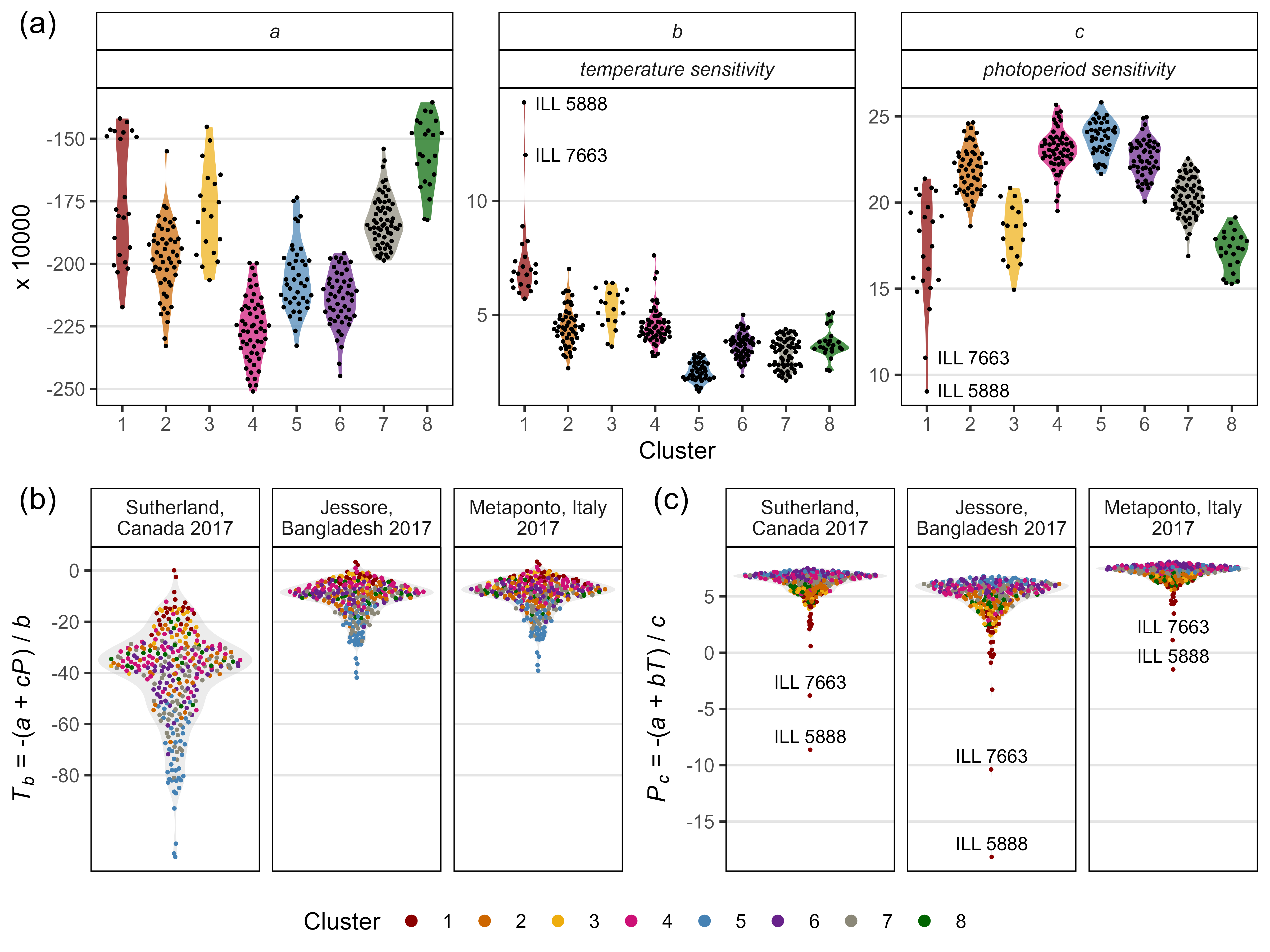
Figure 5: Photothermal constants along with nominal base temperatures and photoperiods for a lentil (Lens culinaris Medik.) diversity panel. (a) Distribution of a, b and c constants calculated from equation 1 among cluster groups. Estimates of: (b) nominal base temperature (Tb), and (c) nominal base photoperiod (Pc) based on equations 2 and 3, respectively, using the mean temperature (T) and photoperiod (P) from Sutherland, Canada 2017, Jessore, Bangladesh 2017 and Metaponto, Italy 2017.
# Prep data for (a) a, b and c
pca <- read.csv("data/data_pca_results.csv") %>%
  select(Entry, Cluster) %>%
  mutate(Cluster = factor(Cluster))
xx <- read.csv("data/model_t+p_coefs.csv") %>%
  left_join(pca, by = "Entry") %>%
  select(Entry, Name, Cluster, a, b, c) %>%
  gather(Constant, Value, 4:ncol(.)) %>%
  mutate(Meaning = plyr::mapvalues(Constant, c("a","b","c"),
           c("", "temperature sensitivity", "photoperiod sensitivity")))
x1 <- xx %>% filter(Entry %in% c(94,105), Constant != "a") %>%
  mutate(Name = gsub(" AGL", "", Name))
# Plot (a) a, b and c
mp1 <- ggplot(xx, aes(x = Cluster, y = Value * 10000) ) +
  geom_violin(aes(fill = Cluster), color = NA, alpha = 0.7) +
  geom_quasirandom(size = 0.3) +
  geom_text_repel(data = x1, aes(label = Name), size = 3, nudge_x = 0.5) +
  facet_wrap(Constant + Meaning ~ ., nrow = 1, scales = "free") +
  theme_AGL +
  theme(strip.text = element_text(face = "italic"),
        legend.position = "none", panel.grid.major.x = element_blank()) +
  scale_fill_manual(name = NULL, values = colors) +
  guides(fill = F) +
  labs(y = "x 10000")
# Prep data
xx <- read.csv("data/data_tb_pc.csv") %>%
  left_join(pca, by = "Entry") %>%
  mutate(Expt = factor(Expt, levels = names_Expt)) %>%
  select(Entry, Name, Expt, ExptShort, Cluster, Tb, Pc, predicted_Tf, predicted_Pf)
x1 <- xx %>%
  filter(ExptShort %in% c("Su17", "Ba17", "It17")) %>%
  group_by(Entry, Name, Expt, ExptShort, Cluster) %>%
  summarise_at(vars(Tb, Pc), funs(mean), na.rm = T)
# Plot (b) Tb
mp2.1 <- ggplot(x1, aes(x = 1, y = Tb, group = Expt)) +
  geom_violin(fill = "grey", alpha = 0.3, color = NA) +
  geom_quasirandom(aes(color = Cluster), size = 0.3) +
  facet_grid(. ~ Expt, labeller = label_wrap_gen(width = 17)) +
  scale_y_continuous(breaks = seq(-80,0,20), minor_breaks = seq(-110,0,10)) +
  scale_color_manual(values = colors) +
  theme_AGL +
  theme(axis.text.x  = element_blank(),
        axis.ticks.x = element_blank(),
        panel.grid.major.x = element_blank()) +
  guides(colour = guide_legend(nrow = 1, override.aes = list(size=2))) +
  labs(y = expression(paste(italic("T")[italic("b")], " = -(", italic("a"), " + ",
              italic("cP"), ") / ", italic("b"))), x = NULL)
# Plot (c) Pc
x2 <- x1 %>%
  filter(Entry %in% c(94,105)) %>%
  ungroup() %>%
  mutate(Name = gsub(" AGL", "", Name))
mp2.2 <- ggplot(x1, aes(x = 1, y = Pc, group = Expt)) +
  geom_violin(fill = "grey", alpha = 0.3, color = NA) +
  geom_quasirandom(aes(color = Cluster), size = 0.3) +
  facet_grid(. ~ Expt, labeller = label_wrap_gen(width = 17)) +
  geom_text(data = x2, aes(label = Name), size = 3, nudge_y = 1.2) +
  scale_y_continuous(breaks = c(-20,-15,-10,-5,0,5)) +
  scale_color_manual(values = colors) +
  theme_AGL +
  theme(axis.text.x        = element_blank(),
        axis.ticks.x       = element_blank(),
        panel.grid.major.x = element_blank()) +
  guides(colour = guide_legend(nrow = 1, override.aes = list(size=2))) +
  labs(y = expression(paste(italic("P")[italic("c")], " = -(", italic("a"), " + ",
             italic("bT"), ") / ", italic("c"))), x = NULL)
mp2 <- ggarrange(mp2.1, mp2.2, nrow = 1, ncol = 2,
                 common.legend = T, legend = "bottom",
                 labels = c("(b)","(c)"), font.label = list(face = "plain"))
#
mp <- ggarrange(mp1, mp2, nrow = 2, ncol = 1, align = "hv",
                labels = c("(a)",""), font.label = list(face = "plain"))
ggsave("Figure_05.png", mp, width = 8, height = 6, dpi = 600, bg = "white")
Figure 6: Origin Constants
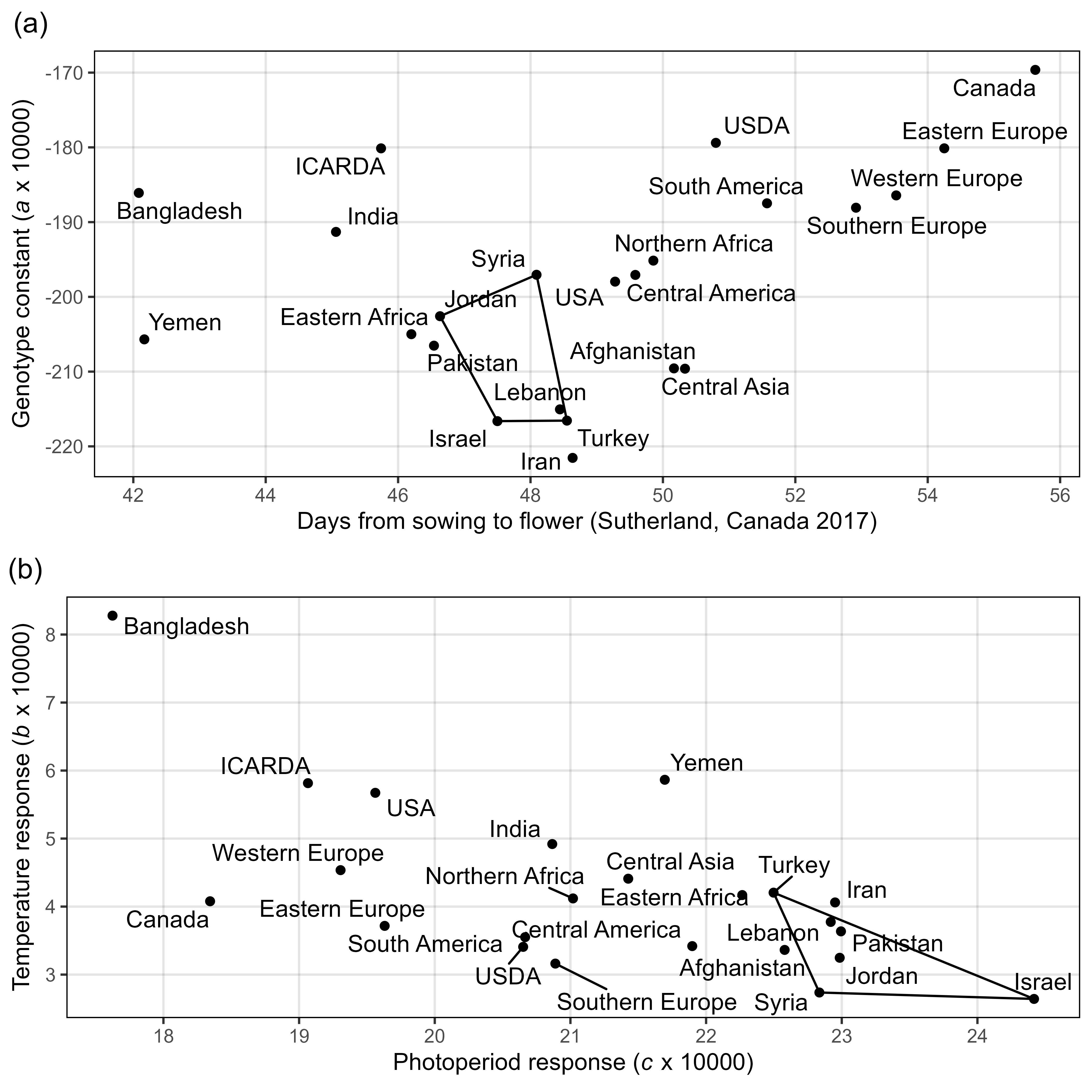
Figure 6: Photothermal responses of lentil (Lens culinaris Medik.) adapted to regions outside the center of origin. (a) Comparison of days from sowing to flowering in Sutherland, Canada 2017 and the genotype constant a (x 104) derived from equation 1. (b) Comparison of temperature response (b x 104) and photoperiod response (c x 104) derived from equation 1. Polygons represent the variation inherent in the region where the crop was domesticated.
# Prep data
mycts <- c("Canada", "USA", "Iran", "Yemen",
           "India", "Pakistan", "Bangladesh", "Afghanistan",
           "Syria", "Jordan", "Turkey", "Lebanon", "Israel")
xx <- read.csv("data/model_t+p_coefs.csv") %>%
  left_join(select(ldp, Entry, Origin), by = "Entry") %>%
  left_join(select(ct, Origin=Country, SubRegion), by = "Origin") %>%
  filter(Origin != "Unknown") %>%
  mutate(SubRegion = as.character(SubRegion), Origin = as.character(Origin),
         SubRegion = ifelse(Origin %in% c("ICARDA", "USDA"),
                            Origin, as.character(SubRegion)),
         Origin = ifelse(Origin %in% mycts, Origin, as.character(SubRegion)))
x1 <- xx %>%
  left_join(dd %>% filter(ExptShort == "Su17") %>%
              select(Entry, DTF), by = "Entry") %>%
  group_by(Origin) %>%
  summarise_at(vars(DTF, a, b, c), funs(mean, sd)) %>%
  filter(Origin != "Unknown")
x2 <- x1 %>% mutate(CO = 1) %>%
  filter(Origin %in% c("Syria", "Jordan", "Turkey", "Lebanon", "Israel"))
# Plot (a) a vs DTF
find_hull <- function(df) df[chull(df[,"DTF_mean"], df[,"a_mean"]), ]
polys <- plyr::ddply(x2, "CO", find_hull)
mp1 <- ggplot(x1, aes(x = DTF_mean, y = a_mean * 10000)) +
  geom_polygon(data = polys, fill = NA, color = "black") +
  geom_point() +
  geom_text_repel(aes(label = Origin)) +
  scale_x_continuous(breaks = seq(42, 56, 2)) +
  theme_AGL +
  theme(plot.title = element_text(hjust = -0.085) ) +
  labs(title = "(a)",
       y = expression(paste("Genotype constant (", italic(a)," x 10000)")),
       x = "Days from sowing to flower (Sutherland, Canada 2017)")
# Plot (b) b vs c
find_hull <- function(df) df[chull(df[,"c_mean"], df[,"b_mean"]), ]
polys <- plyr::ddply(x2, "CO", find_hull)
mp2 <- ggplot(x1, aes(x = c_mean * 10000, y = b_mean * 10000)) +
  geom_polygon(data = polys, fill = NA, color = "black") +
  geom_point() +
  geom_text_repel(aes(label = Origin)) +
  scale_x_continuous(breaks = seq(18, 24, 1)) +
  scale_y_continuous(breaks = 3:8) +
  theme_AGL +
  theme(plot.title = element_text(hjust = -0.06) ) +
  labs(title = "(b)",
       y = expression(paste("Temperature response (", italic(b), " x 10000)")),
       x = expression(paste("Photoperiod response (", italic(c), " x 10000)")))
# Append (a) and (b)
mp <- ggarrange(mp1, mp2, ncol = 1, nrow = 2)
ggsave("Figure_06.png", mp, width = 7, height = 7, dpi = 600)
ggsave("Additional/Temp/Temp_F06_1.png", mp1, width = 8, height = 4, dpi = 600)
ggsave("Additional/Temp/Temp_F06_2.png", mp2, width = 8, height = 4, dpi = 600)
Supplemental Figure 9: Pc Tf PTT
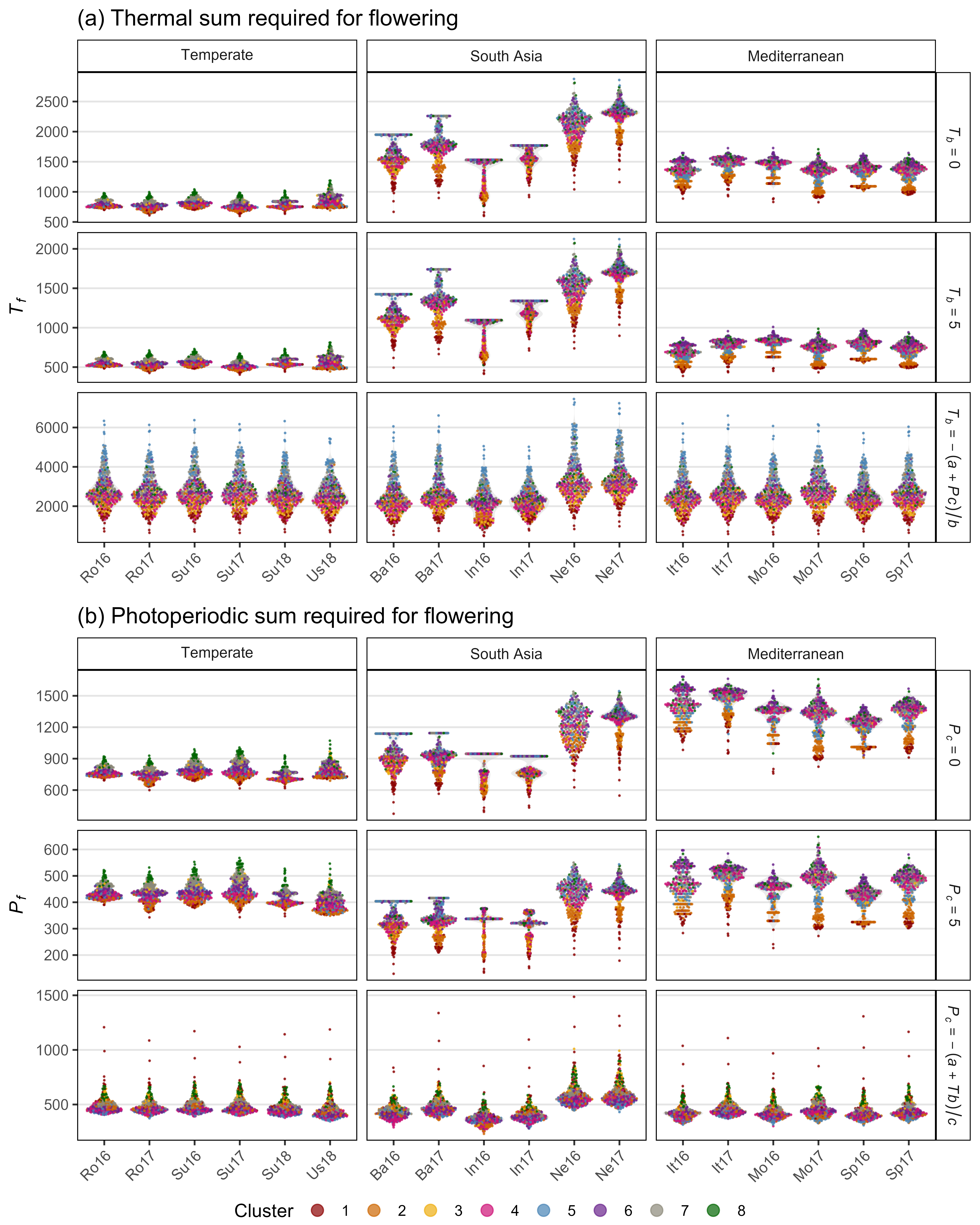
Figure S9: (a) Thermal sum required for flowering (Tf), using a base temperature (Tb) of 0°C, 5°C and calculated using equation 3, across all site-years. (b) Photoperiodic sum required for flowering (Pf), using a critical photoperiod (Pc) of 0h, 5h and calculated using equation 4, across all site-years. Rosthern, Canada 2016 and 2017 (Ro16, Ro17), Sutherland, Canada 2016, 2017 and 2018 (Su16, Su17, Su18), Central Ferry, USA 2018 (Us18), Metaponto, Italy 2016 and 2017 (It16, It17), Marchouch, Morocco 2016 and 2017 (Mo16, Mo17), Cordoba, Spain 2016 and 2017 (Sp16, Sp17), Bhopal, India 2016 and 2017 (In16, In17), Jessore, Bangladesh 2016 and 2017 (Ba16, Ba17), Bardiya, Nepal 2016 and 2017 (Ne16, Ne17).
# Prep data for (a) Tf
pca <- read.csv("data/data_pca_results.csv") %>%
  select(Entry, Cluster) %>%
  mutate(Cluster = factor(Cluster))
xx <- read.csv("data/data_tb_pc.csv") %>%
  left_join(pca, by = "Entry") %>%
  mutate(MacroEnv = factor(MacroEnv, levels = names_MacroEnvs))
x1 <- xx %>%
  select(Entry, Name, Expt, ExptShort, MacroEnv, Cluster, Tf_0, Tf_5, Tf) %>%
  gather(Trait, Value, Tf_0, Tf_5, Tf) %>%
  mutate(Trait = factor(Trait, levels = c("Tf_0", "Tf_5", "Tf")))
new.lab <- as_labeller(c(
  Tf_0 = "italic(T)[italic(b)]==0", Tf_5 = "italic(T)[italic(b)]==5",
  Tf = "italic(T)[italic(b)]==-(italic(a)+italic(Pc))/italic(b)",
  Mediterranean = "Mediterranean", Temperate = "Temperate",
  `South Asia` = "South~Asia"), label_parsed)
# Plot (a) Tf
mp1 <- ggplot(x1, aes(x = ExptShort, y = Value, group = Expt)) +
  geom_violin(fill = "grey", alpha = 0.3, color = NA) +
  geom_quasirandom(aes(color = Cluster), size = 0.1, alpha = 0.7) +
  facet_grid(Trait ~ MacroEnv, scales = "free", labeller = new.lab) +
  scale_color_manual(values = colors) +
  theme_AGL +
  theme(legend.position = "bottom",
        legend.margin = unit(c(0,0,0,0), "cm"),
        panel.grid.major.x = element_blank(),
        axis.text.x = element_text(angle = 45, hjust = 1)) +
  guides(colour = guide_legend(nrow = 1, override.aes = list(size = 3))) +
  labs(title = "(a) Thermal sum required for flowering",
       y = expression(italic("T")[italic("f")]), x = NULL)
# Prep data for B) Pf
x1 <- xx %>%
  select(Entry, Expt, ExptShort, MacroEnv, Cluster, Pf_0, Pf_7, Pf) %>%
  gather(Trait, Value, Pf_0, Pf_7, Pf) %>%
  mutate(Trait = factor(Trait, levels = c("Pf_0", "Pf_7", "Pf")))
new.lab <- as_labeller(c(
  Pf_0 = "italic(P)[italic(c)]==0", Pf_7 = "italic(P)[italic(c)]==5",
  Pf = "italic(P)[italic(c)]==-(italic(a)+italic(Tb))/italic(c)",
  Mediterranean = "Mediterranean", Temperate = "Temperate",
  `South Asia` = "South~Asia"), label_parsed)
# Plot (b) Pf
mp2 <- ggplot(x1, aes(x = ExptShort, y = Value, group = Expt)) +
  geom_violin(fill = "grey", alpha = 0.3, color = NA) +
  geom_quasirandom( aes(color = Cluster), size = 0.1, alpha = 0.7) +
  facet_grid(Trait ~ MacroEnv, scales = "free", labeller = new.lab) +
  scale_color_manual(values = colors) +
  theme_AGL +
  theme(legend.position = "bottom",
        legend.margin = unit(c(0,0,0,0), "cm"),
        panel.grid.major.x = element_blank(),
        axis.text.x = element_text(angle = 45, hjust = 1)) +
  guides(colour = guide_legend(nrow = 1, override.aes = list(size = 3))) +
  labs(title = "(b) Photoperiodic sum required for flowering",
       y = expression(italic("P")[italic("f")]), x = NULL)

# Append (a), (b) and (c)
mp <- ggarrange(mp1, mp2, ncol = 1, common.legend = T, legend = "bottom")
# Save
ggsave("Additional/Temp/Temp_SF09_1.png", mp1, width = 8, height = 6, dpi = 600)
ggsave("Additional/Temp/Temp_SF09_2.png", mp2, width = 8, height = 6, dpi = 600)
ggsave("Supplemental_Figure_09.png", mp, width = 8, height = 10, dpi = 600, bg = "white")
Additional Figure 14: PTT
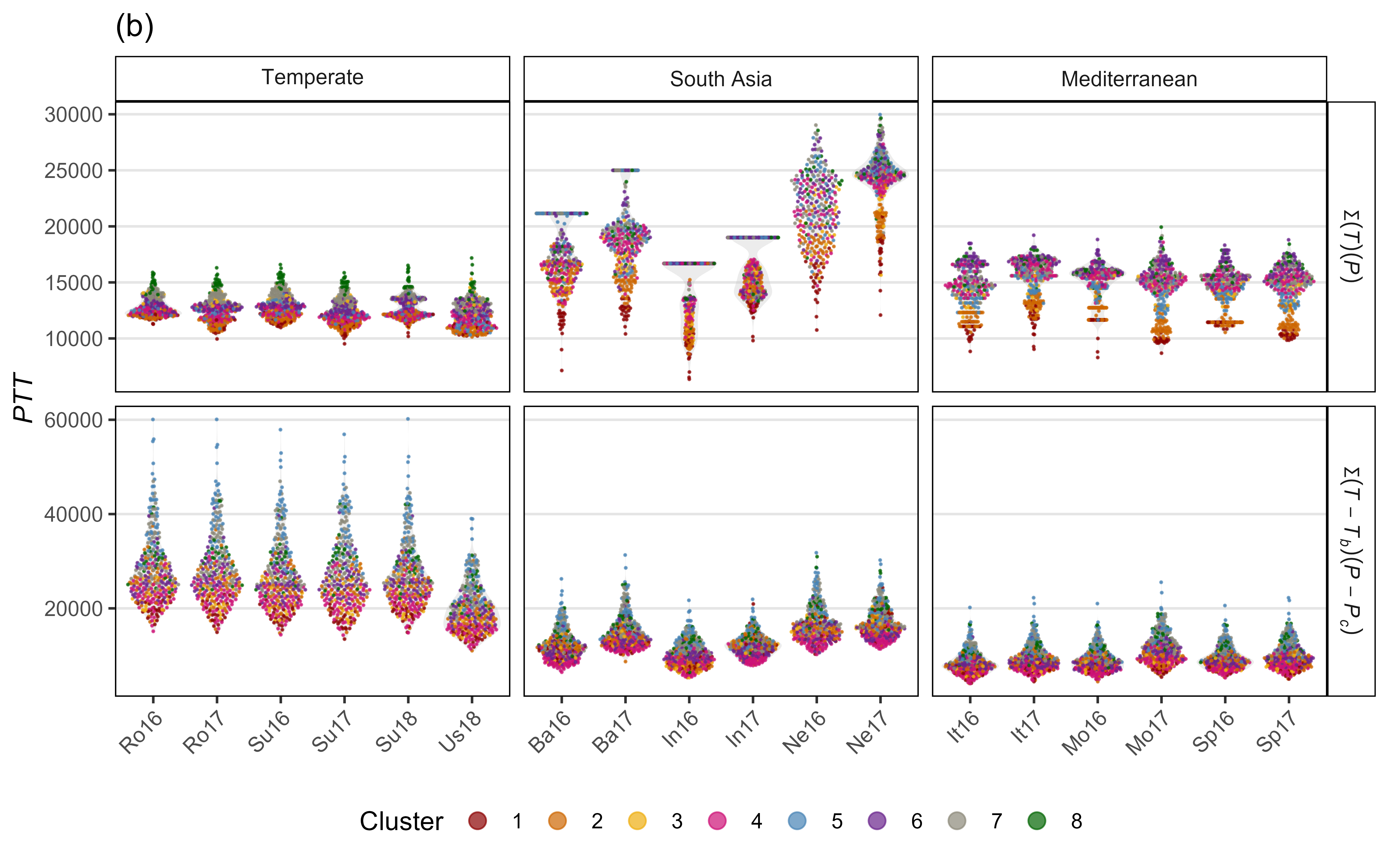
# Prep data
pca <- read.csv("data/data_pca_results.csv") %>%
  select(Entry, Cluster) %>%
  mutate(Cluster = factor(Cluster))
xx <- read.csv("data/data_tb_pc.csv") %>%
  left_join(pca, by = "Entry") %>%
  mutate(MacroEnv = factor(MacroEnv, levels = names_MacroEnvs)) %>%
  select(Entry, Expt, ExptShort, MacroEnv, Cluster, PTT_0, PTT) %>%
  gather(Trait, Value, PTT_0, PTT) %>%
  mutate(Trait = factor(Trait, levels = c("PTT_0", "PTT")))
new.lab <- as_labeller(c(PTT_0 = "Sigma(italic(T))(italic(P))",
  PTT = "Sigma(italic(T)-italic(T)[italic(b)])(italic(P)-italic(P)[italic(c)])",
  Mediterranean = "Mediterranean", Temperate = "Temperate",
  `South Asia` = "South~Asia"), label_parsed)
# Plot PTT
mp <- ggplot(xx, aes(x = ExptShort, y = Value)) +
  geom_violin(fill = "grey", alpha = 0.3, color = NA) +
  geom_quasirandom(aes(color = Cluster), size = 0.1, alpha = 0.7) +
  facet_grid(Trait ~ MacroEnv, scales = "free", labeller = new.lab) +
  scale_color_manual(values = colors) +
  theme_AGL +
  theme(legend.position = "bottom",
        panel.grid.major.x = element_blank(),
        axis.text.x = element_text(angle = 45, hjust = 1)) +
  guides(colour = guide_legend(nrow = 1, override.aes = list(size = 3))) +
  labs(title = "(b)", y = expression(italic("PTT")), x = NULL)
ggsave("Additional/Additional_Figure_14.png", mp, width = 8, height = 5, dpi = 600)
Supplemental Figure 10: Thermal Sums
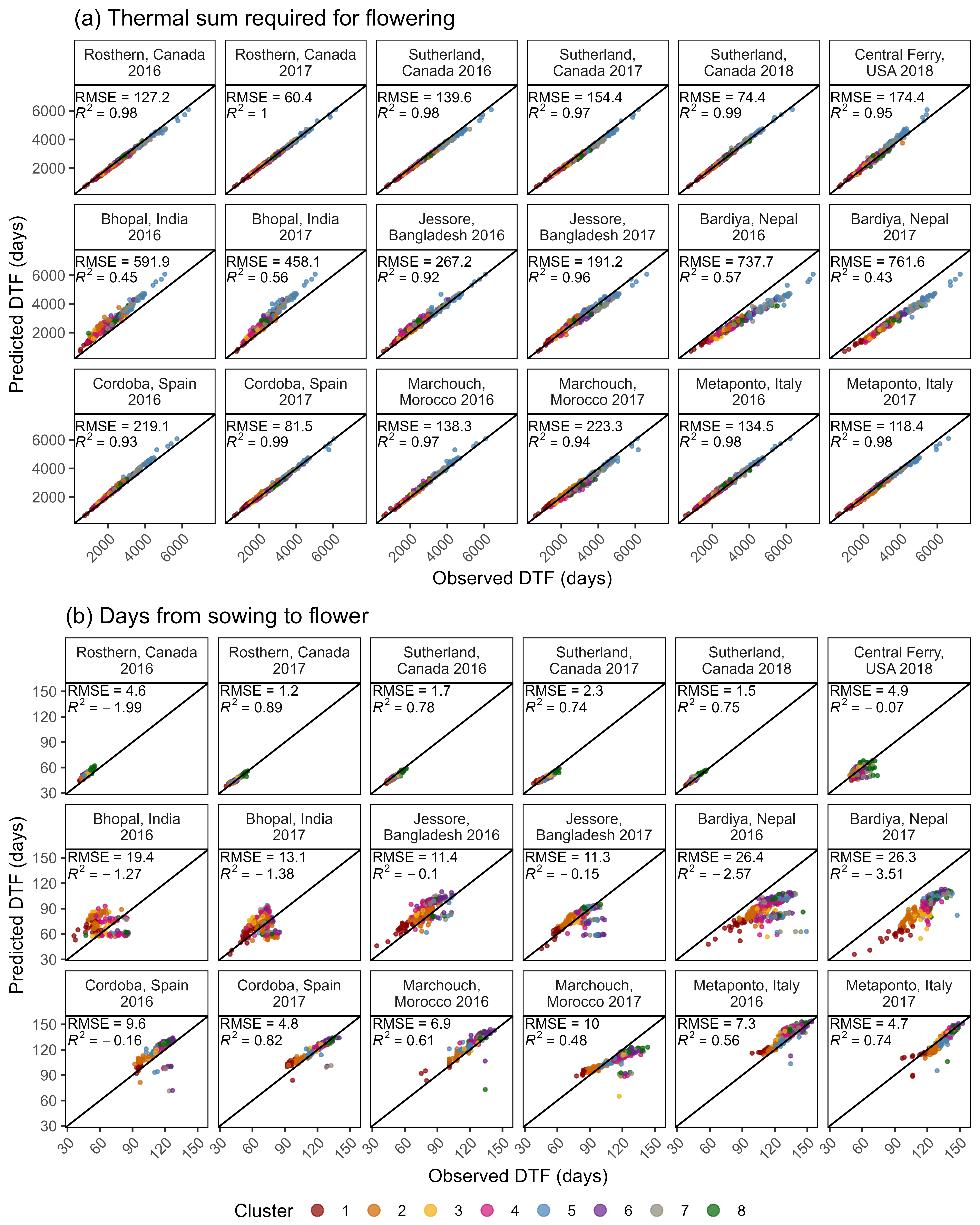
Figure S10: Comparison of observed vs predicted values, along with the coefficient of determination (R2) and root-mean-square error (RMSE), for (a) thermal sum required for flowering and (b) days from sowing to flowering, calculated using equation 5.
# Prep data
xx <- read.csv("data/data_tb_pc.csv") %>%
  mutate(Expt = factor(Expt, levels = names_Expt))
# Plot (a)
mp1 <- ggModel2(xx, "Tf", "predicted_Tf",
                "(a) Thermal sum required for flowering",
                200, 200, 6600, 5500)
# Plot (b)
mp2 <- ggModel2(xx, "DTF", "predicted_DTF_Tf",
                "(b) Days from sowing to flower",
                30, 30, 145, 125)
# Append (a) and (b)
mp <- ggarrange(mp1, mp2, nrow = 2, ncol = 1,
                common.legend = T, legend = "bottom")
ggsave("Supplemental_Figure_10.png", mp, width = 8, height = 10, dpi = 600, bg = "white")
Supplemental Figure 11: Photoperiodic Sums
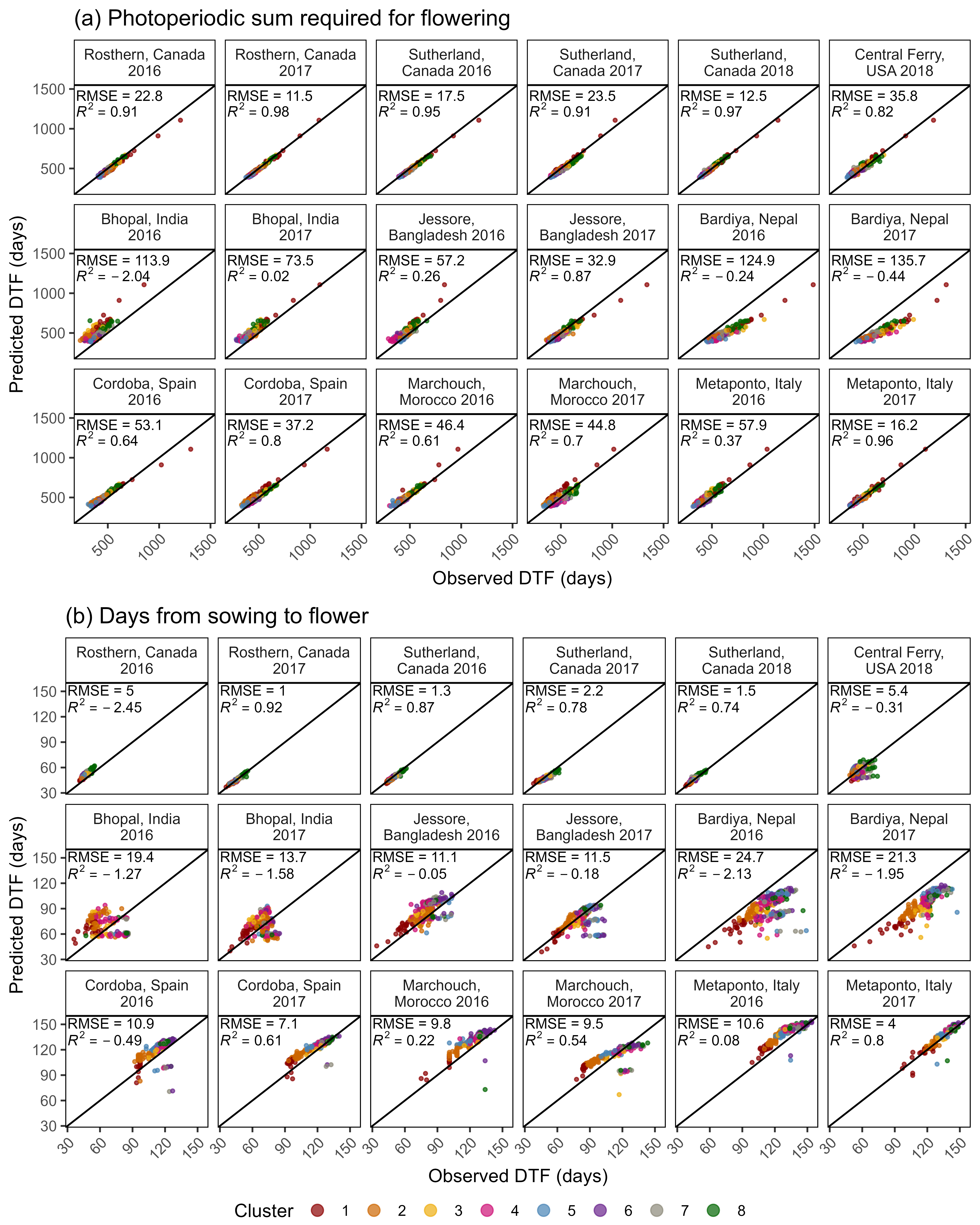
Figure S11: Comparison of observed vs predicted values, along with the coefficient of determination (R2) and root-mean-square error (RMSE) for (a) photoperiodic sum required for flowering and (b) days from sowing to flowering, calculated using equation 6.
# Prep data
xx <- read.csv("data/data_tb_pc.csv") %>%
  mutate(Expt = factor(Expt, levels = names_Expt))
# Plot (a)
mp1 <- ggModel2(xx, "Pf", "predicted_Pf",
                "(a) Photoperiodic sum required for flowering",
                190, 190, 1350, 1150)
# Plot (b)
mp2 <- ggModel2(xx, "DTF", "predicted_DTF_Pf",
                "(b) Days from sowing to flower",
                30, 30, 145, 125)
# Append (a) and (b)
mp <- ggarrange(mp1, mp2, nrow = 2, ncol = 1,
                common.legend = T, legend = "bottom")
ggsave("Supplemental_Figure_11.png", mp, width = 8, height = 10, dpi = 600, bg = "white")
Figure 7: Temperature Increase By MacroEnv
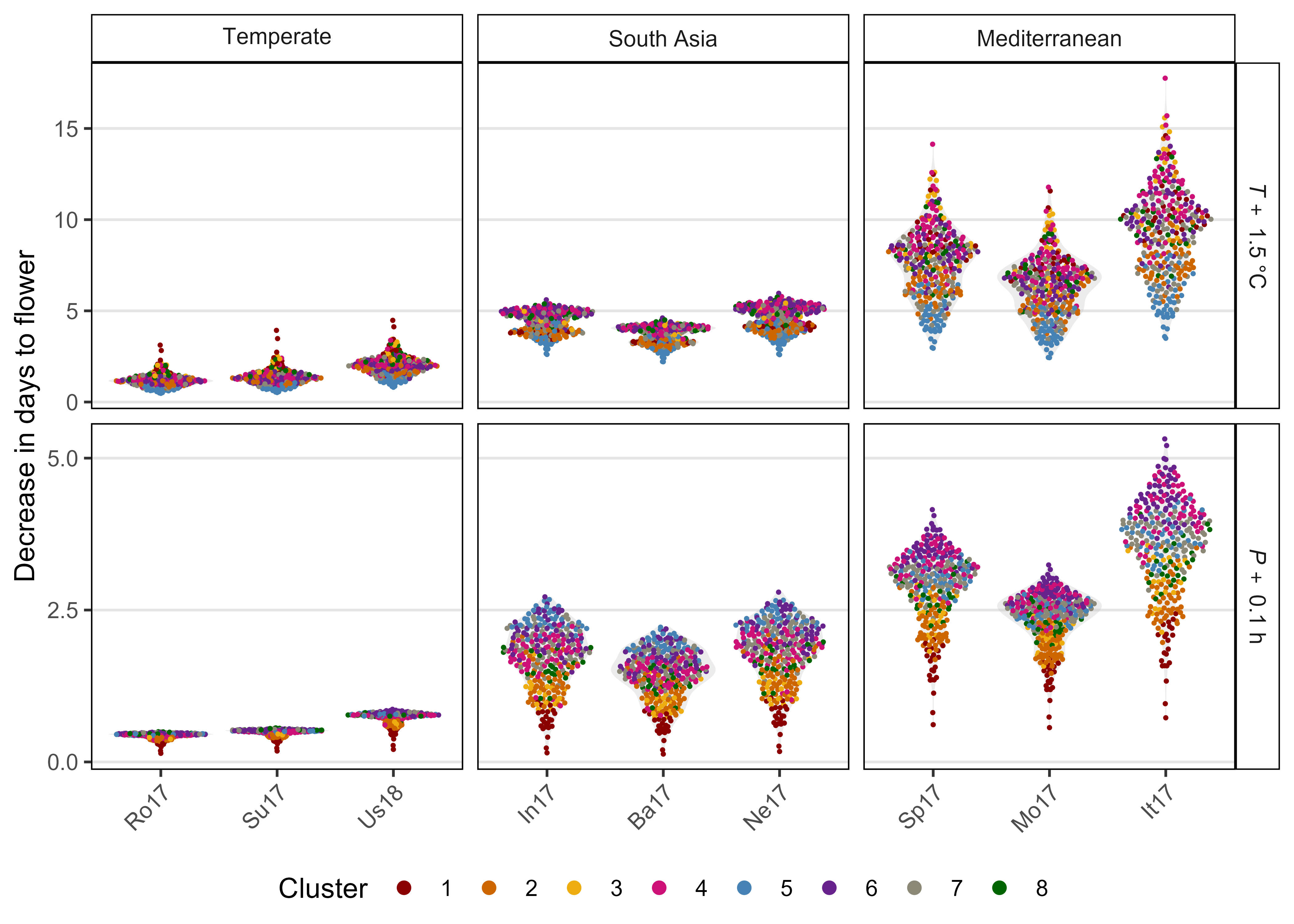
Figure 7: Predicted decrease in days from sowing to flowering for a lentil (Lens culinaris Medik.) diversity panel based on a mean temperature (T) or photoperiod (P) increases of 1.5oC or 0.1h using equation 1 in the selected locations: Rosthern, Canada 2017 (Ro17), Sutherland, Canada 2017 (Su17), Central Ferry, USA 2018 (Us18), Bhopal, India 2017 (In17), Jessore, Bangladesh 2017 (Ba17), Bardiya, Nepal 2017 (Ne17), Marchouch, Morocco 2017 (Mo17), Cordoba, Spain 2017 (Sp17) and Metaponto, Italy 2017 (It17).
# Prep data
yy <- c("Ro17", "Su17", "Us18", "In17", "Ba17", "Ne17", "Sp17", "Mo17", "It17")
coefs <- read.csv("data/model_t+p_coefs.csv")
pca <- read.csv("data/data_pca_results.csv") %>%
  select(Entry, Cluster) %>%
  mutate(Cluster = factor(Cluster))
xx <- dd %>%
  select(Entry, Expt, ExptShort, DTF) %>%
  left_join(coefs, by = "Entry") %>%
  left_join(pca, by = "Entry") %>%
  left_join(select(ff, Expt, MacroEnv, T_mean, P_mean), by = "Expt")
# Temp +1
x1 <- xx %>%
  mutate(T_mean_1.5 = T_mean + 1.5,
         DTF_1 = 1 / (a + b * T_mean_1.5 + c * P_mean),
         DTF_0  = 1 / (a + b * T_mean + c * P_mean),
         Difference = DTF_0 - DTF_1) %>%
  filter(ExptShort %in% yy)
x2 <- xx %>%
  mutate(P_mean_0.1 = P_mean + 0.1,
         DTF_1 = 1 / (a + b * T_mean + c * P_mean_0.1),
         DTF_0  = 1 / (a + b * T_mean + c * P_mean),
         Difference = DTF_0 - DTF_1) %>%
  filter(ExptShort %in% yy)
x1 <- x1 %>% mutate(Treatment = "T + 1.5")
x2 <- x2 %>% mutate(Treatment = "P + 0.1")
knitr::kable(x1 %>% group_by(MacroEnv) %>%
summarise(Min = round(min(Difference), 2), Max = round(max(Difference), 2)) )| MacroEnv | Min | Max |
|---|---|---|
| Temperate | 0.48 | 4.48 |
| South Asia | 2.21 | 5.96 |
| Mediterranean | 2.43 | 17.76 |
knitr::kable(x2 %>% group_by(MacroEnv) %>%
summarise(Min = round(min(Difference), 2), Max = round(max(Difference), 2)) )| MacroEnv | Min | Max |
|---|---|---|
| Temperate | 0.14 | 0.87 |
| South Asia | 0.13 | 2.79 |
| Mediterranean | 0.57 | 5.32 |
xx <- bind_rows(x1, x2) %>%
  select(Expt, ExptShort, MacroEnv, Entry, Name, Cluster,
         DTF_0, DTF_1, Difference, Treatment) %>%
  mutate(Treatment = factor(Treatment, levels = c("T + 1.5", "P + 0.1")))
write.csv(xx, "data/data_temp_photo_increase.csv", row.names = F)
new.lab <- as_labeller(c(`T + 1.5` = "italic(T)~+~1.5~degree*C",
    `P + 0.1` = "italic(P)~+~0.1~h", Mediterranean = "Mediterranean",
    Temperate = "Temperate", `South Asia` = "South~Asia"), label_parsed)
my_breaks <- function(x) { if (max(x) < 6) c(0,2.5,5) else seq(0,30,5) }
# Plot
mp <- ggplot(xx, aes(x = ExptShort, y = Difference, group = Expt)) +
  geom_violin(fill = "grey", alpha = 0.3, color = NA) +
  geom_quasirandom(aes(color = Cluster), size = 0.3) +
  facet_grid(Treatment ~ MacroEnv, scales = "free", labeller = new.lab) +
  scale_y_continuous(minor_breaks = 0:30, breaks = my_breaks) +
  scale_color_manual(values = colors) +
  theme_AGL +
  theme(legend.position = "bottom",
        legend.margin = unit(c(0,0,0,0), "cm"),
        axis.text.x = element_text(angle = 45, hjust = 1),
        panel.grid.major.x = element_blank()) +
  guides(colour = guide_legend(nrow = 1, override.aes = list(size=2))) +
  labs(y = "Decrease in days to flower", x = NULL)
ggsave("Figure_07.png", mp, width = 7, height = 5, dpi = 600)
© Derek Michael Wright