gg_Manhattan_Zoom()
2.2_gg_Manhattan_Zoom.RmdDue to the large size of most genomes, small shifts in the x-axis on a standard manhattan plot can result in large distances.
The function gg_Manhattan_Zoom() creates manhattan plots
from GAPIT GWAS results zoomed into a specific region on a
chromosome.
Specifying a folder, a trait and a
chr (defaults to 1 if not specified) is all that is needed
to create zoomed in manhattan plots.
# Plot
mp <- gg_Manhattan_Zoom(
  # Specify a folder with GWAS results
  folder = "GWAS_Results/",
  # Select a trait to plot
  trait = "Cotyledon_RedvsYellow",
  # Plot just Chromosome 1
  chr = 1 )
# Save
ggsave("figures/gg_Manhattan_Zoom_01.png", mp, width = 6, height = 4, bg = "white")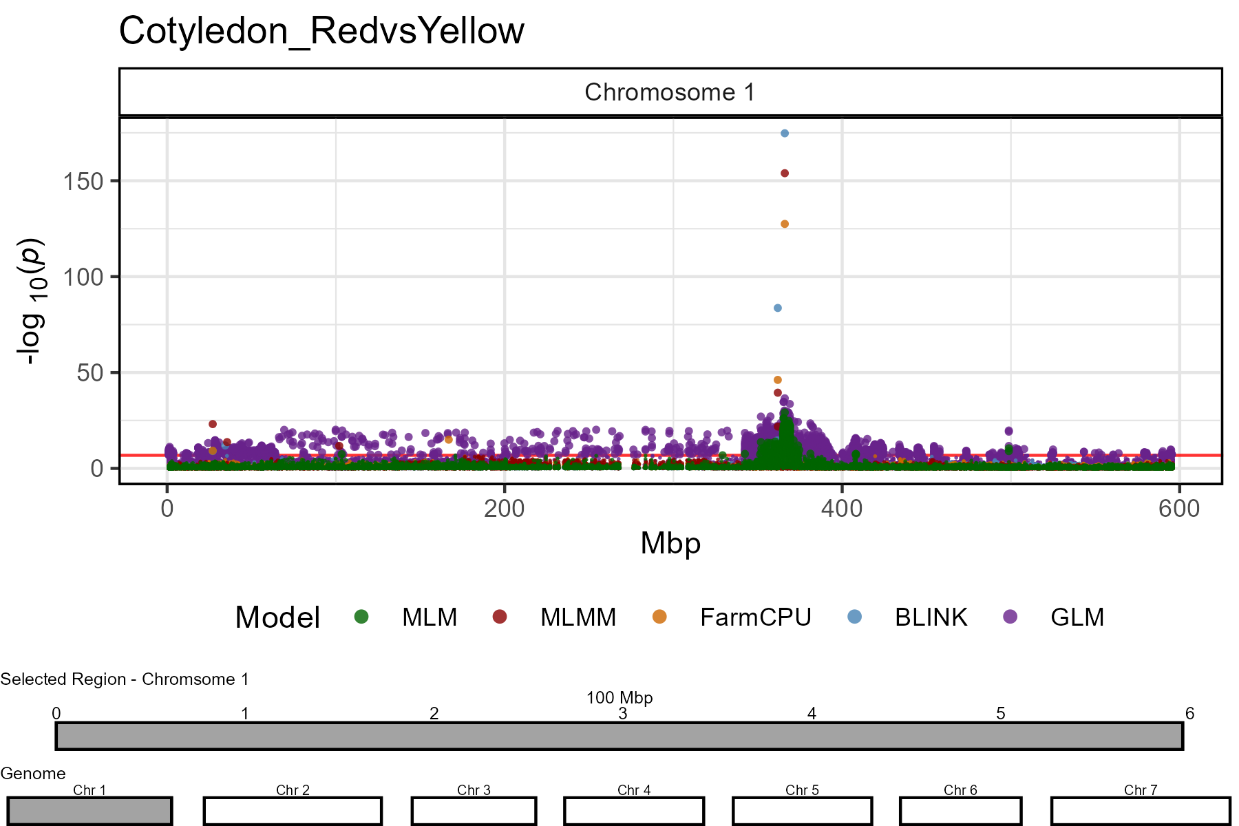
Facet by Model
The default for gg_Manhattan_Zoom() is to set
facet = F and plot all GWAS models together. However, if
facet = T, then the different GWAS models can be
separated.
# Plot
mp <- gg_Manhattan_Zoom(
  # Specify a folder with GWAS results
  folder = "GWAS_Results/",
  # Select a trait to plot
  trait = "Cotyledon_RedvsYellow",
  # Plot just Chromosome 1
  chr = 1,
  # Should models be facetted
  facet = T )
# Save
ggsave("figures/gg_Manhattan_Zoom_02.png", mp, width = 6, height = 8, bg = "white")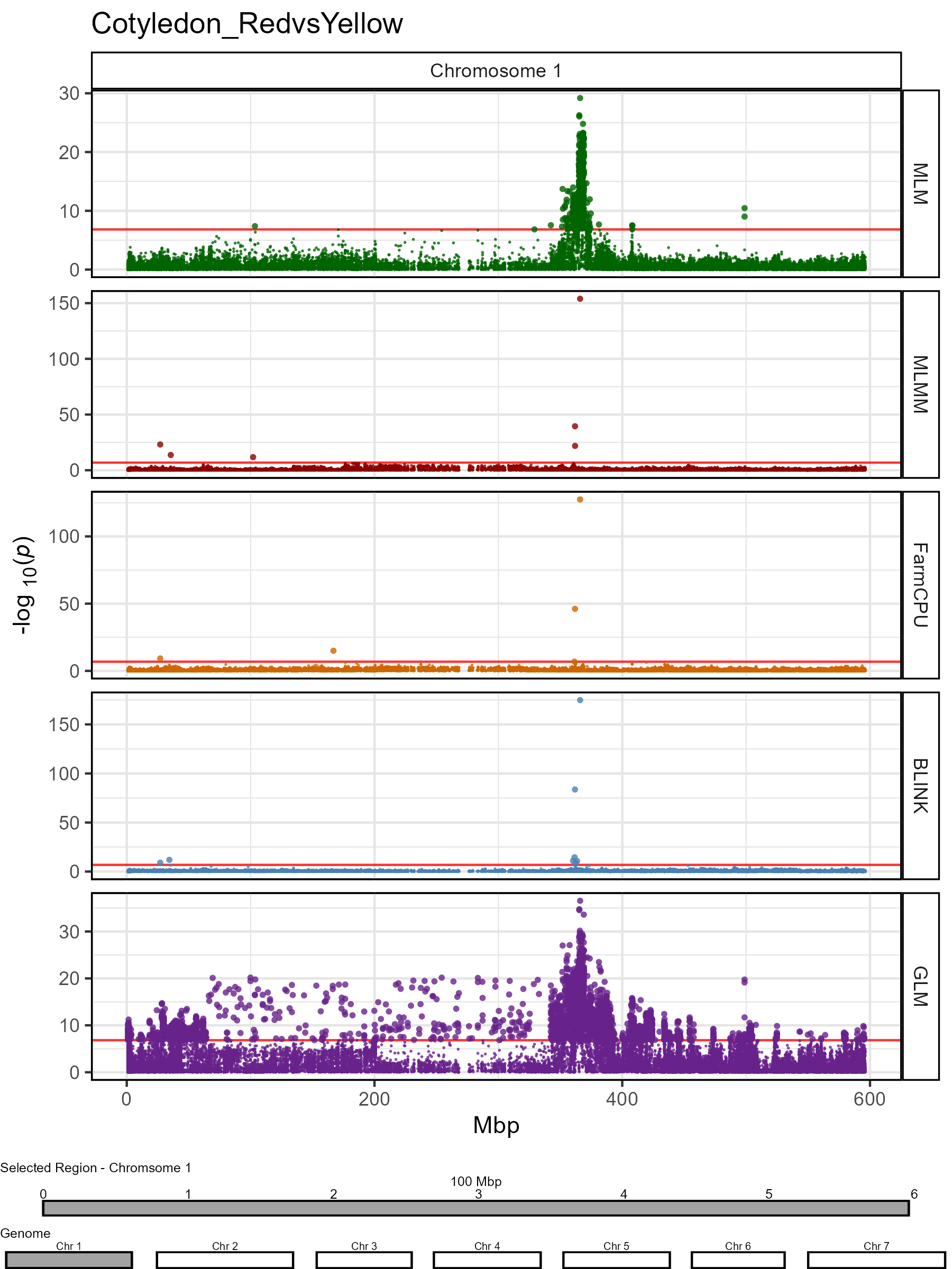
Customized Plots
Any Region within a chromosome can be plotted by specifying
pos1 and pos2.
# Plot
mp <- gg_Manhattan_Zoom(
  # Specify a folder with GWAS results
  folder = "GWAS_Results/",
  # Select a trait to plot
  trait = "Cotyledon_RedvsYellow",
  # Plot just Chromosome 1
  chr = 1,
  pos1 = 350000000,
  pos2 = 400000000,
  # Highlight specific markers
  markers = c("Lcu.1GRN.Chr1p365986872",
              "Lcu.1GRN.Chr1p361840399"),
  # Create alt labels for the markers
  labels = c("365Mbp","361Mbp"),
  # Specify Color for each marker vline
  vline.colors = c("red", "blue"),
  # Should models be facetted
  facet = T )
# Save
ggsave("figures/gg_Manhattan_Zoom_03.png", mp, width = 6, height = 8, bg = "white")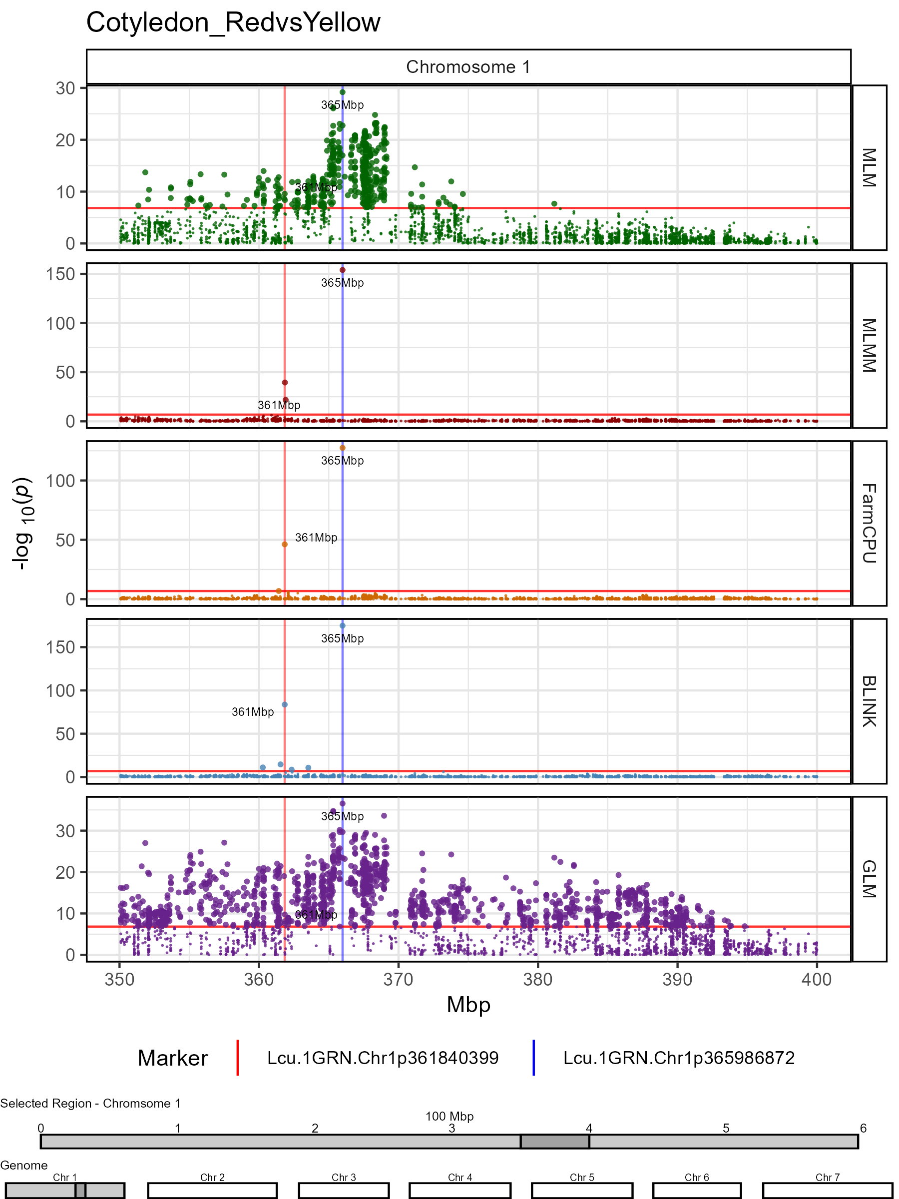
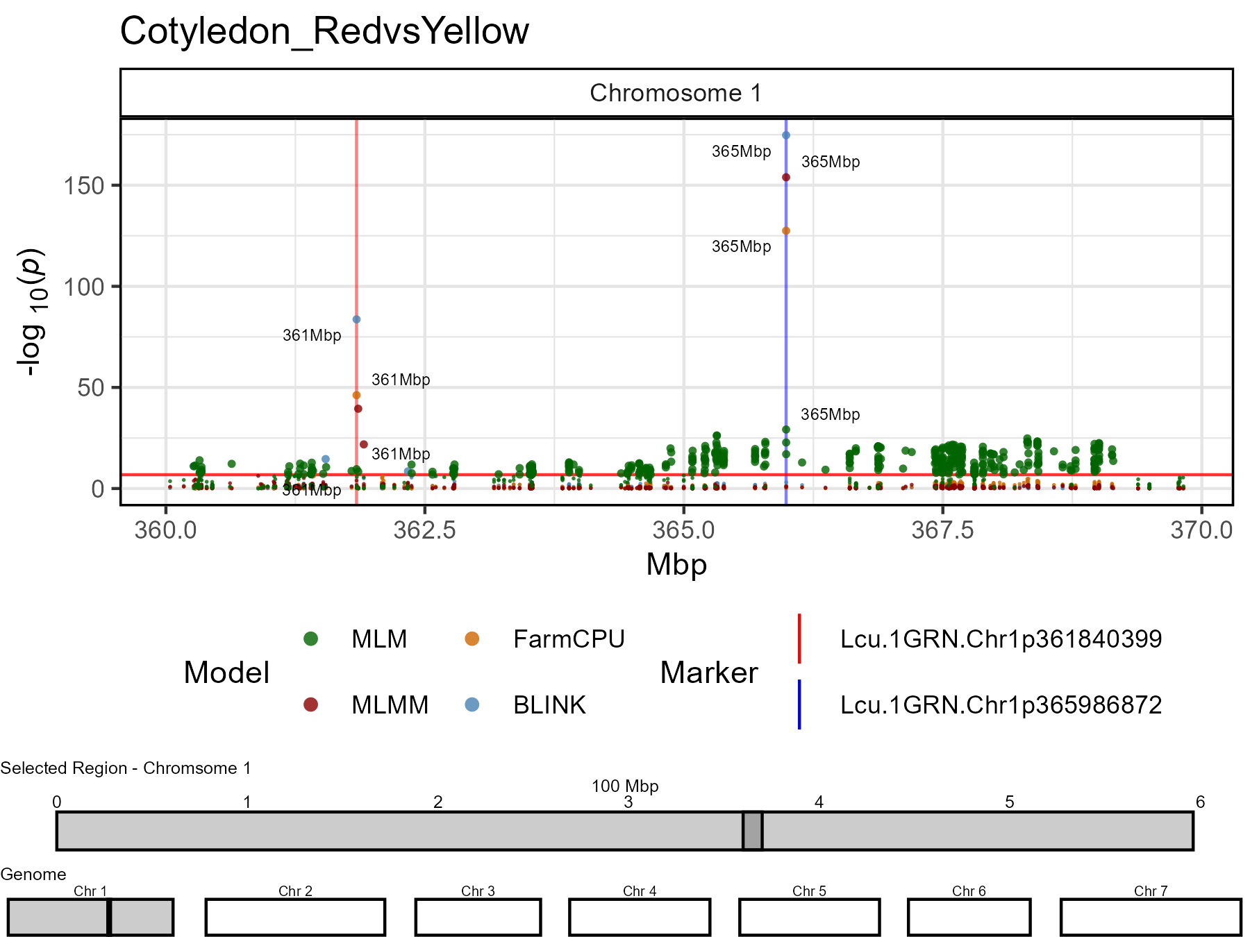
# Plot
mp <- gg_Manhattan_Zoom(
  # Specify a folder with GWAS results
  folder = "GWAS_Results/",
  # Select a trait to plot
  trait = "Cotyledon_RedvsYellow",
  # Plot just Chromosome 1
  chr = 1,
  pos1 = 360000000,
  pos2 = 370000000,
  # Highlight specific markers
  markers = c("Lcu.1GRN.Chr1p365986872",
              "Lcu.1GRN.Chr1p361840399"),
  # Create alt labels for the markers
  labels = c("365Mbp","361Mbp"),
  # Specify Color for each marker vline
  vline.colors = c("red", "blue"),
  # Should models be facetted
  facet = T )
# Save
ggsave("figures/gg_Manhattan_Zoom_04.png", mp, width = 6, height = 8, bg = "white")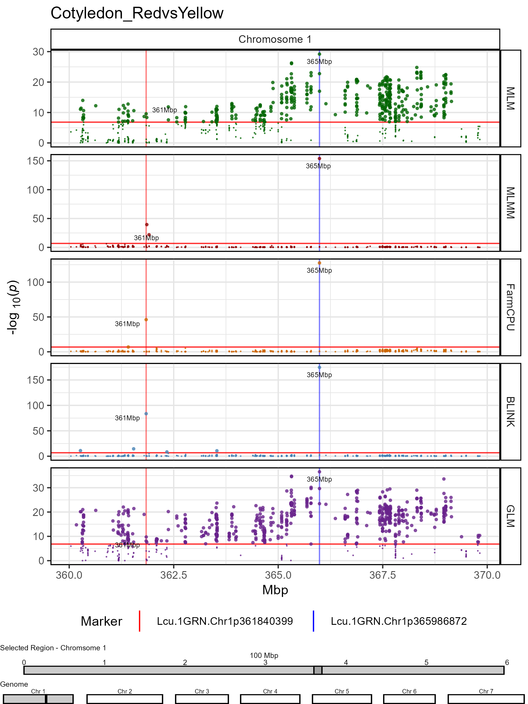
If there are markers with extremely high -log10(p) values,
pmax can be set to make plots more readable.
# Plot
mp <- gg_Manhattan_Zoom(
  # Specify a folder with GWAS results
  folder = "GWAS_Results/",
  # Select a trait to plot
  trait = "Cotyledon_RedvsYellow",
  # Plot just Chromosome 1
  chr = 1,
  pos1 = 360000000,
  pos2 = 370000000,
  # Plot only certain GWAS models
  models = c("MLM","MLMM","FarmCPU","BLINK"),
  # Set colors for each GWAS model
  model.colors = c("darkgreen","darkred", "darkorange3", "steelblue"),
  # Highlight specific markers
  markers = c("Lcu.1GRN.Chr1p365986872",
              "Lcu.1GRN.Chr1p361840399"),
  # Create alt labels for the markers
  labels = c("365Mbp","361Mbp"),
  # Specify Color for each marker vline
  vline.colors = c("red", "blue"),
  # Set the number of rows in the legend
  legend.rows = 2,
  # Should models be facetted
  facet = F
  # set a max P value
  #pmax = 40
  )
# Save
ggsave("figures/gg_Manhattan_Zoom_05.png", mp, width = 6, height = 4.5, bg = "white")