The function gg_LD_Decay() creates Linkage
Disequilibrium (LD) Decay plots from GAPIT GWAS results.
Specifying a myG object, an outputFolder,
and a markerNum is all that is needed to calculate and plot
LD decay.
Note: this is a computation heavy function and the larger you set
markerNumthe longer the computation will take. Start by setting to a lower number such as200which is the default.
# Load genotype file (note: header = T)
myG <- read.csv("gwaspr_myG_hmp.csv", header = T)
markerNum = 200
# Calulate LD decay
calc_LD_Decay(
  # Load genotype data
  xG = myG,
  # Specify a folder with GWAS results
  outputFolder = "LD_Decay/",
  # Select the number of markers per chromosome to analyse
  markerNum = 200 )
# Plot
mp <- gg_LD_Decay(
  # Load genotype data
  xG = myG,
  # Specify a folder with GWAS results
  outputFolder = "LD_Decay/",
  # Select the number of markers per chromosome to analyse
  markerNum = 200 )
# Save
ggsave("figures/gg_LD_Decay_01.png", mp, width = 12, height = 10 )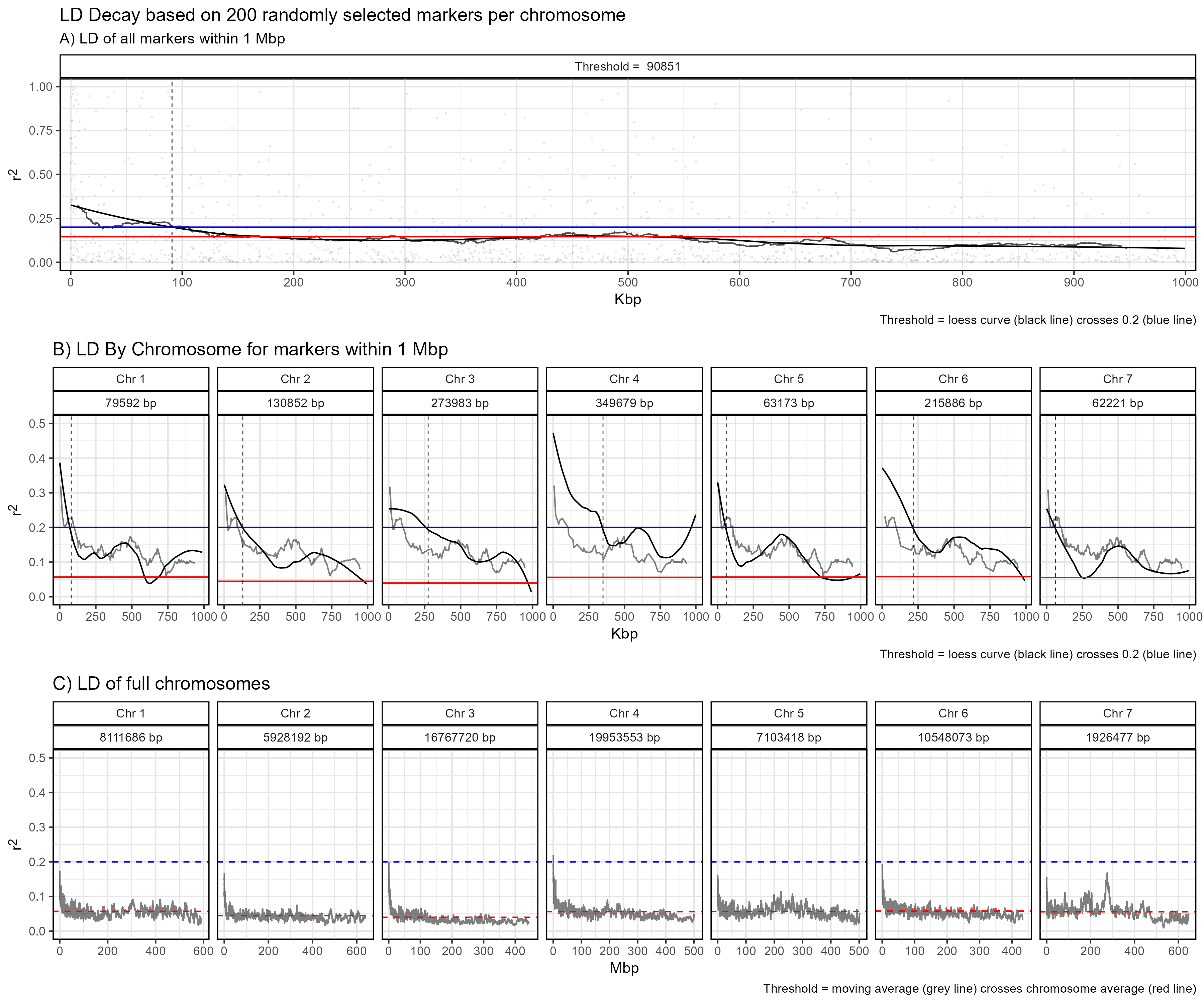
markerNum = 2000
# Calulate LD decay
calc_LD_Decay(
  # Load genotype data
  xG = myG,
  # Specify a folder with GWAS results
  outputFolder = "LD_Decay/",
  # Select the number of markers per chromosome to analyse
  markerNum = 2000 )
# Plot
mp <- gg_LD_Decay(
  # Load genotype data
  xG = myG,
  # Specify a folder with GWAS results
  outputFolder = "LD_Decay/",
  # Select the number of markers per chromosome to analyse
  markerNum = 2000 )
# Save
ggsave("figures/gg_LD_Decay_02.png", mp, width = 12, height = 10 )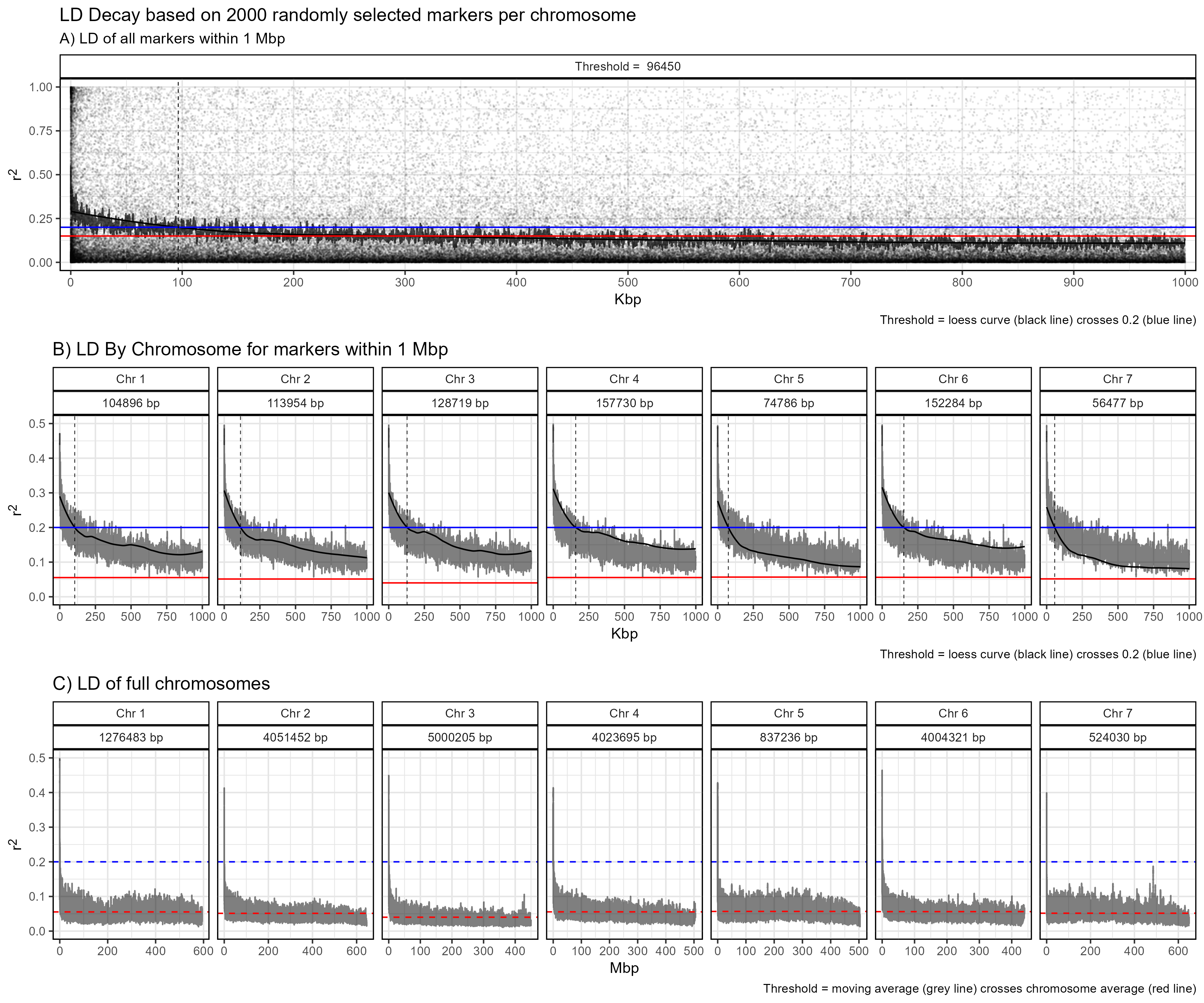
LD Table
The function table_LD_Decay() creates a table
xx <- table_LD_Decay(
  xG = myG,
  outputFolder = "LD_Decay/")
write.csv(xx, "LD_Summary_Table.csv", row.names = F)
## Chr X200 X2000
## 1 1 79592 104896
## 2 2 130852 113954
## 3 3 273983 128719
## 4 4 349679 157730
## 5 5 63173 74786
## 6 6 215886 152284
## 7 7 62221 56477
xx <- xx %>% gather(Num, Value, 2:ncol(.))
# Plot
mp <- ggplot(xx, aes(x = Num, y = Value / 1000, fill = Num)) +
  geom_col(position = "dodge", alpha = 0.8) +
  facet_grid(. ~ Chr) +
  scale_fill_manual(values = gwaspr_Colors) +
  theme_gwaspr_col(legend.position = "bottom",
                   axis.text.x = element_text(angle = 45, hjust = 1)) +
  labs(title = "LD decay", y = "Kbp", x = "Maker Number")
ggsave("figures/gg_LD_Decay_03.png", mp, width = 6, height = 4 )