The functions gg_Marker_Box(),
gg_Marker_Bar(), and gg_Marker_Pie() create
marker plots with your myY and myG GWAS input
files.
Load data
# Load genotype file (note: header = T)
myG <- read.csv("gwaspr_myG_hmp.csv", header = T)
# Map + marker Info
myG[1:10,1:11]
## V1 V2 V3 V4 V5 V6 V7 V8
## 1 rs alleles chrom pos strand assembly center protLSID
## 2 Lcu.1GRN.Chr1p853882 A/G 1 853882 <NA> <NA> <NA> <NA>
## 3 Lcu.1GRN.Chr1p854117 G/A 1 854117 <NA> <NA> <NA> <NA>
## 4 Lcu.1GRN.Chr1p854159 A/C 1 854159 <NA> <NA> <NA> <NA>
## 5 Lcu.1GRN.Chr1p854174 C/G 1 854174 <NA> <NA> <NA> <NA>
## 6 Lcu.1GRN.Chr1p870836 A/G 1 870836 <NA> <NA> <NA> <NA>
## 7 Lcu.1GRN.Chr1p870898 C/T 1 870898 <NA> <NA> <NA> <NA>
## 8 Lcu.1GRN.Chr1p870903 G/A 1 870903 <NA> <NA> <NA> <NA>
## 9 Lcu.1GRN.Chr1p871108 A/G 1 871108 <NA> <NA> <NA> <NA>
## 10 Lcu.1GRN.Chr1p872492 T/C 1 872492 <NA> <NA> <NA> <NA>
## V9 V10 V11
## 1 assayLSID panel QCcode
## 2 <NA> <NA> <NA>
## 3 <NA> <NA> <NA>
## 4 <NA> <NA> <NA>
## 5 <NA> <NA> <NA>
## 6 <NA> <NA> <NA>
## 7 <NA> <NA> <NA>
## 8 <NA> <NA> <NA>
## 9 <NA> <NA> <NA>
## 10 <NA> <NA> <NA>
# genotrype calls
myG[1:10,12:17]
## V12 V13 V14 V15 V16
## 1 X3156.11_AGL CDC_Asterix_AGL CDC_Cherie_AGL CDC_Glamis_AGL CDC_Gold_AGL
## 2 G A G A G
## 3 G G G A G
## 4 C C C C C
## 5 G G G G G
## 6 G G N G G
## 7 T C N C T
## 8 G G N A G
## 9 A A A A A
## 10 T T T T T
## V17
## 1 CDC_Greenstar_AGL
## 2 A
## 3 G
## 4 A
## 5 C
## 6 A
## 7 C
## 8 G
## 9 A
## 10 N
# Load phenotype file
myY <- read.csv("gwaspr_myY.csv")
# Convert our nominal trait from numeric to factor.
myY <- myY %>%
  mutate(Cotyledon_Color = mv(Cotyledon_RedvsYellow, c(1, 0, NA), c("Red", "Yellow", "Green")),
         Cotyledon_Color = factor(Cotyledon_Color, levels = c("Red", "Yellow", "Green")))
myY[1:20,]## Name DTF_Sask_2017 DTF_Nepal_2017 Cotyledon_RedvsYellow
## 1 CDC_Asterix_AGL 54.7 128.0 0
## 2 CDC_Rosie_AGL 59.0 123.3 1
## 3 X3156.11_AGL 60.7 125.3 1
## 4 CDC_Greenstar_AGL 56.7 121.0 0
## 5 CDC_Cherie_AGL 54.3 125.3 1
## 6 CDC_Glamis_AGL 59.0 123.0 0
## 7 CDC_Gold_AGL 54.0 125.3 0
## 8 CDC_Imax_AGL 53.0 128.7 1
## 9 CDC_Impower_AGL 57.0 123.3 0
## 10 CDC_KR.1_AGL 57.0 121.7 1
## 11 CDC_LeMay_AGL 55.7 126.7 0
## 12 CDC_Maxim_AGL 54.3 125.7 1
## 13 CDC_QG.1_AGL 57.7 126.7 NA
## 14 CDC_Red_Rider_AGL 57.0 123.5 1
## 15 CDC_Redcoat_AGL 57.7 126.7 1
## 16 CDC_Redwing_AGL 57.3 128.7 1
## 17 CDC_Robin_AGL 52.0 124.7 1
## 18 CDC_Rosebud_AGL 54.7 121.3 1
## 19 CDC_Rosetown_AGL 57.7 123.7 1
## 20 CDC_Rouleau_AGL 55.3 123.7 1
## Cotyledon_Color
## 1 Yellow
## 2 Red
## 3 Red
## 4 Yellow
## 5 Red
## 6 Yellow
## 7 Yellow
## 8 Red
## 9 Yellow
## 10 Red
## 11 Yellow
## 12 Red
## 13 Green
## 14 Red
## 15 Red
## 16 Red
## 17 Red
## 18 Red
## 19 Red
## 20 Redgg_Marker_Box
Single marker, single trait
Specifying a trait and a marker along with
your genotype and phenotype data as xG and xY
is needed to create marker plots.
# Plot
mp <- gg_Marker_Box(
  # Genotype data
  xG = myG,
  # Phenotype data
  xY = myY,
  # Select traits to plot
  traits = "DTF_Sask_2017",
  # Select markers to plot
  markers = "Lcu.1GRN.Chr6p3269280" )
# Save
ggsave("figures/gg_Marker_Box_01.png",
       mp, width = 6, height = 4 )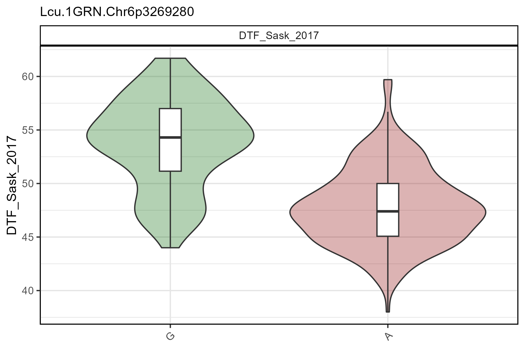
Customized Plots
Boxplots
# Plot
mp <- gg_Marker_Box(
  # Genotype data
  xG = myG,
  # Phenotype data
  xY = myY,
  # Select traits to plot
  traits = "DTF_Sask_2017",
  # Select markers to plot
  markers = "Lcu.1GRN.Chr6p3269280",
  # Select marker colors
  marker.colors = c("darkorange3", "steelblue"),
  # Choose what should be plotted
  plot.violin = F,
  plot.box = T,
  plot.points = F,
  # Change the width of the boxplots
  box.width = 0.3,
  # Create a custom label for the y-axis
  yLab = "Days from sowing to flower" )
# Save
ggsave("figures/gg_Marker_Box_02.png",
       mp, width = 6, height = 4 )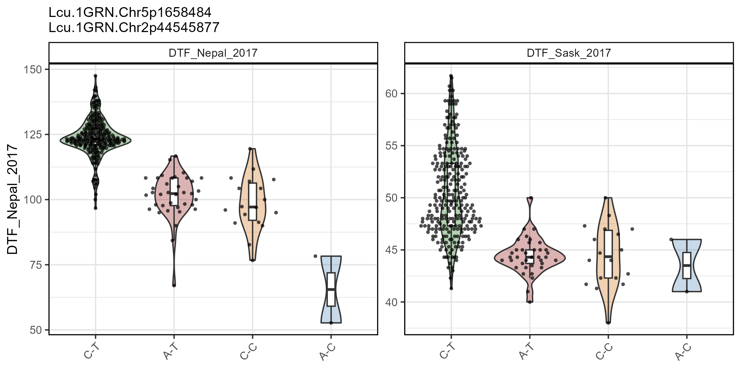
Violin + points
# Plot
mp <- gg_Marker_Box(
  # Genotype data
  xG = myG,
  # Phenotype data
  xY = myY,
  # Select traits to plot
  traits = "DTF_Sask_2017",
  # Select markers to plot
  markers = "Lcu.1GRN.Chr6p3269280",
  # Select marker colors
  marker.colors = c("darkorange3", "steelblue"),
  # Choose what should be plotted
  plot.violin = T,
  plot.box = F,
  plot.points = T,
  # Set the point size
  point.size = 2,
  # Create a custom label for the y-axis
  yLab = "Days from sowing to flower" )
# Save
ggsave("figures/gg_Marker_Box_03.png",
       mp, width = 6, height = 4 )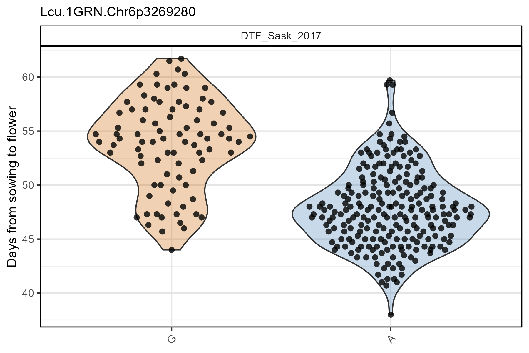
Covariable Point Color
myG covariable
# Plot
mp <- gg_Marker_Box(
  # Genotype data
  xG = myG,
  # Phenotype data
  xY = myY,
  # Select traits to plot
  traits = "DTF_Sask_2017",
  # Select markers to plot
  markers = "Lcu.1GRN.Chr6p3269280",
  # Select marker colors
  marker.colors = c("darkorange3", "darkseagreen4", "steelblue", "burlywood4"),
  # Keep heterozygous markers
  remove.hets = F,
  # Choose what should be plotted
  plot.violin = T,
  plot.box = F,
  plot.points = T,
  # Set the point size
  point.size = 0.75,
  # Plot with geom_beeswarm instead of quasirandom
  point.beeswarm = T,
  # Select Covariable trait for points
  cv.name = "Lcu.1GRN.Chr2p44545877",
  # Select colors for the covariable
  cv.colors = c("darkslategray4", "maroon3", "purple3"),
  # Set a custom label for the covariable legend
  cv.label = "Chr2p44545877" )
# Save
ggsave("figures/gg_Marker_Box_04.png",
       mp, width = 6, height = 4 )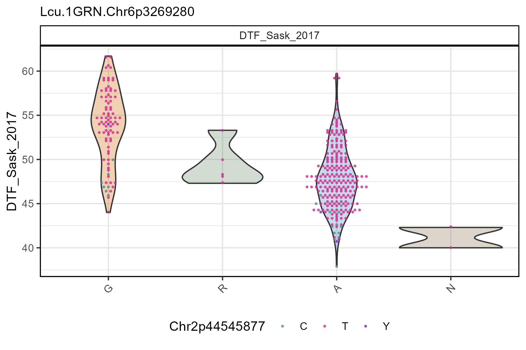
myY covariable
# Plot
mp <- gg_Marker_Box(
  # Genotype data
  xG = myG,
  # Phenotype data
  xY = myY,
  # Select traits to plot
  traits = "DTF_Sask_2017",
  # Select markers to plot
  markers = "Lcu.1GRN.Chr6p3269280",
  # Select marker colors
  marker.colors = c("darkorange3", "steelblue"),
  # Choose what should be plotted
  plot.violin = T,
  plot.box = F,
  plot.points = T,
  # Set the point size
  point.size = 1.5,
  # Plot with geom_beeswarm instead of quasirandom
  point.beeswarm = T,
  # Select covariable source
  cv.source = "xY",
  # Select Covariable trait for points
  cv.name = "Cotyledon_Color",
  # Select colors for the covariable
  cv.colors = c("darkred", "darkgoldenrod2", "darkgreen"),
  # Set a custom label for the covariable legend
  cv.label = "Cotyledon Color" )
# Save
ggsave("figures/gg_Marker_Box_05.png",
       mp, width = 6, height = 4 )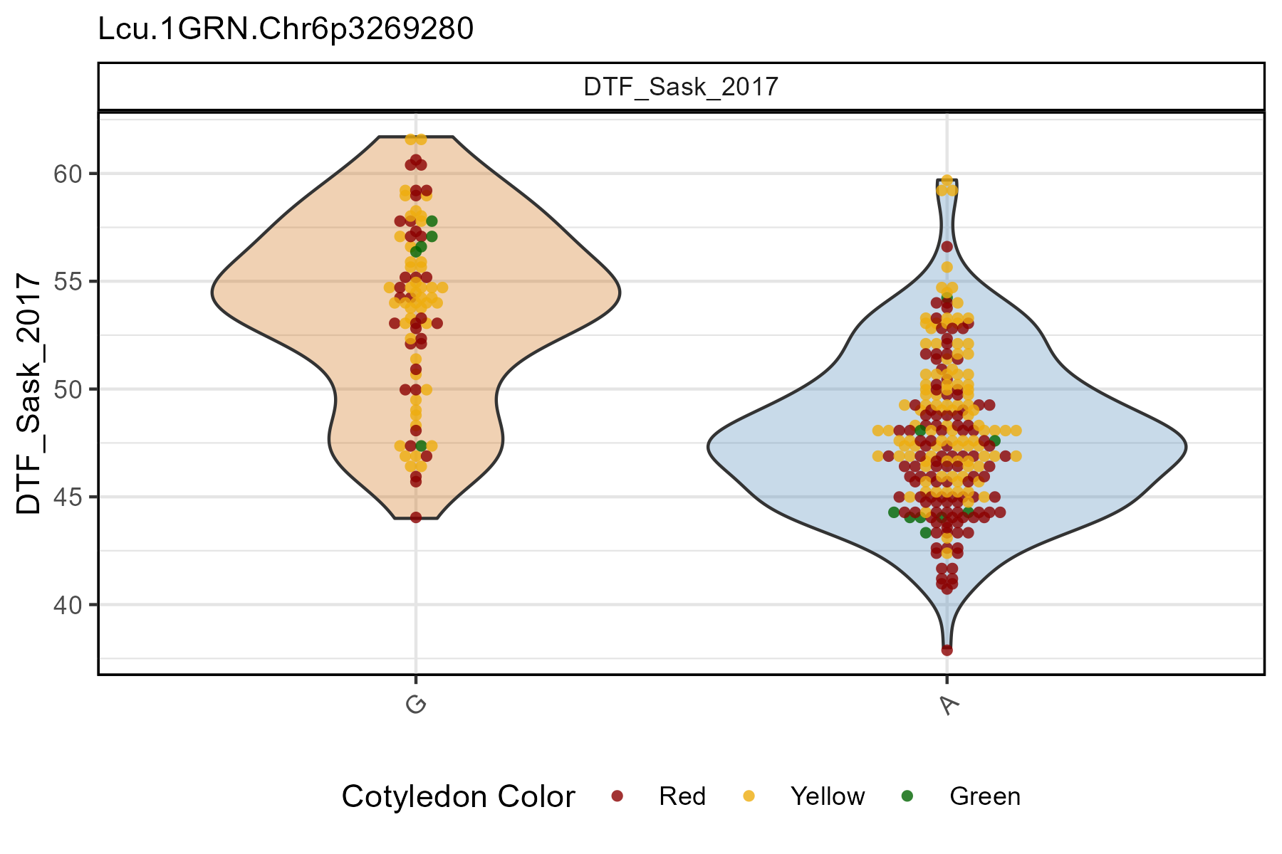
Grouped by myY covariable
# Plot
mp <- gg_Marker_Box(
  # Genotype data
  xG = myG,
  # Phenotype data
  xY = myY,
  # Select traits to plot
  traits = "DTF_Sask_2017",
  # Select markers to plot
  markers = "Lcu.1GRN.Chr6p3269280",
  # Select marker colors
  marker.colors = c("darkorange3", "steelblue"),
  # Choose what should be plotted
  plot.violin = T,
  plot.box = F,
  plot.points = T,
  # Set the point size
  point.size = 1.5,
  # Plot with geom_beeswarm instead of quasirandom
  point.beeswarm = T,
  # Select covariable source
  cv.source = "xY",
  # Select Covariable trait for points
  cv.name = "Cotyledon_Color",
  # Select colors for the covariable
  cv.colors = c("darkred", "darkgoldenrod2", "darkgreen"),
  # Set a custom label for the covariable legend
  cv.label = "Cotyledon Color",
  # Plot CV on x-axis instead of marker
  groupByCV = T)
# Save
ggsave("figures/gg_Marker_Box_06.png",
       mp, width = 6, height = 4 )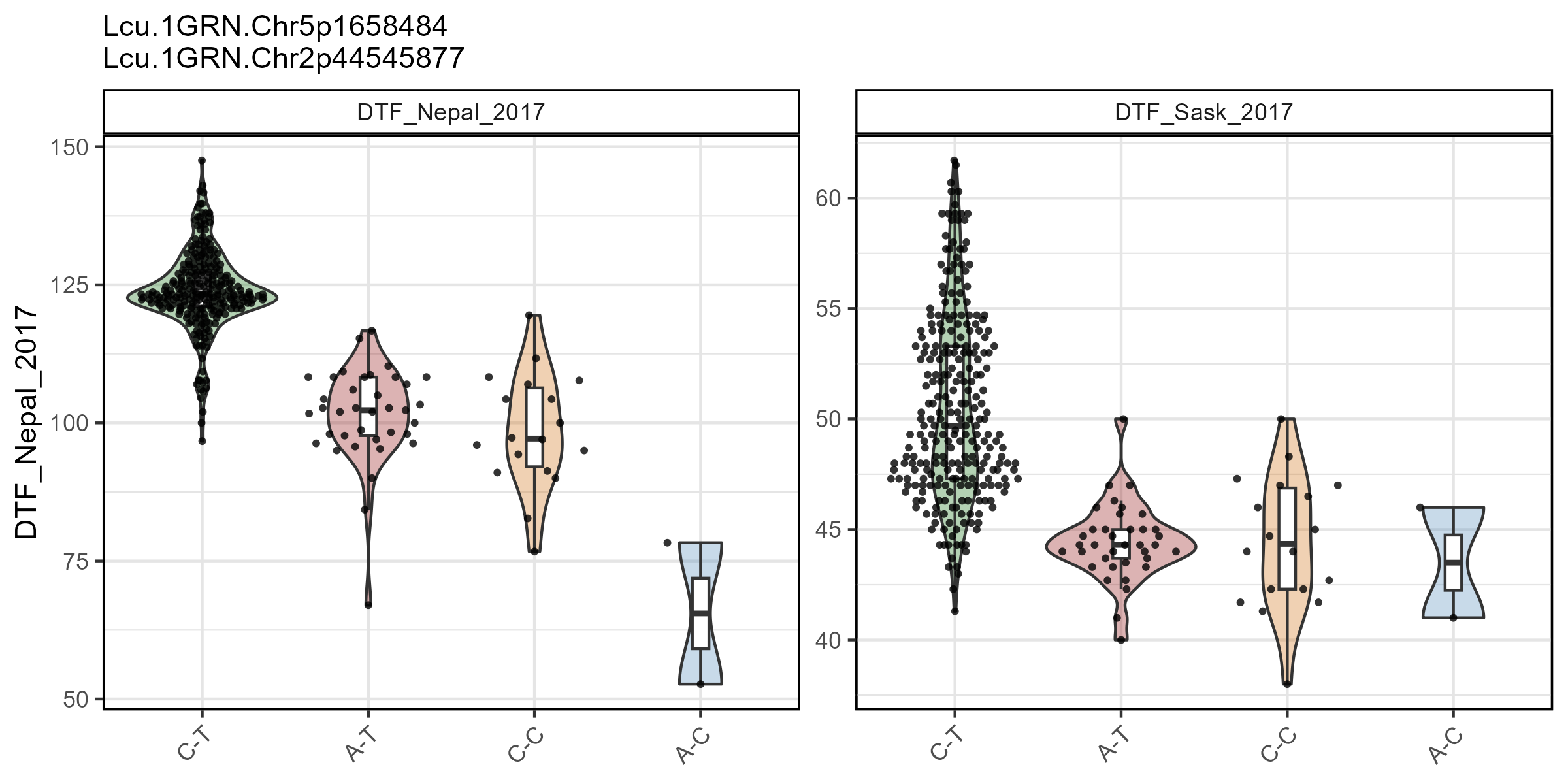
Multiple markers, multiple traits
# Plot
mp <- gg_Marker_Box(
  # Genotype data
  xG = myG,
  # Phenotype data
  xY = myY,
  # Select traits to plot
  traits = c("DTF_Nepal_2017", "DTF_Sask_2017"),
  # Select markers to plot
  markers = c("Lcu.1GRN.Chr5p1658484", "Lcu.1GRN.Chr2p44545877") )
# Save
ggsave("figures/gg_Marker_Box_07.png",
       mp, width = 8, height = 4 )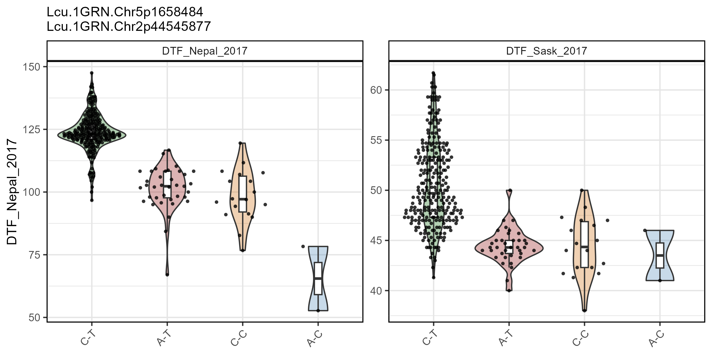
gg_Marker_Bar
Single marker, single trait
# Plot
mp <- gg_Marker_Bar(
  # Genotype data
  xG = myG,
  # Phenotype data
  xY = myY,
  # Select traits to plot
  traits = "DTF_Sask_2017",
  # Select markers to plot
  markers = "Lcu.1GRN.Chr6p3269280" )
# Save
ggsave("figures/gg_Marker_Bar_01.png",
       mp, width = 6, height = 4 )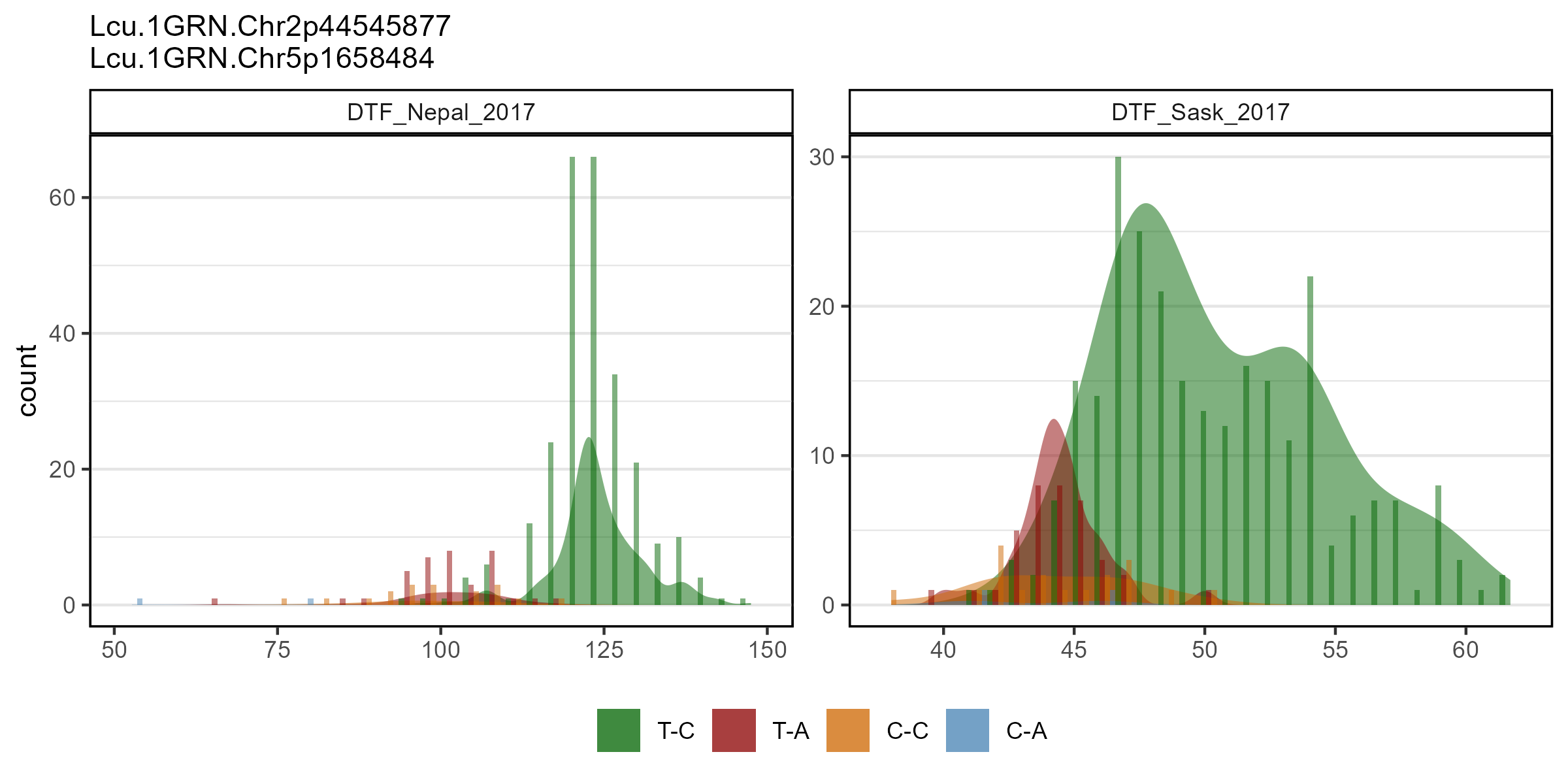
Customized Plots
Histogram
# Plot
mp <- gg_Marker_Bar(
  # Genotype data
  xG = myG,
  # Phenotype data
  xY = myY,
  # Select traits to plot
  traits = "DTF_Sask_2017",
  # Select markers to plot
  markers = "Lcu.1GRN.Chr6p3269280",
  # Select marker colors
  marker.colors = c("darkorange3", "steelblue"),
  # Choose what should be plotted
  plot.histogram = T,
  plot.density = F )
# Save
ggsave("figures/gg_Marker_Bar_02.png",
       mp, width = 6, height = 4 )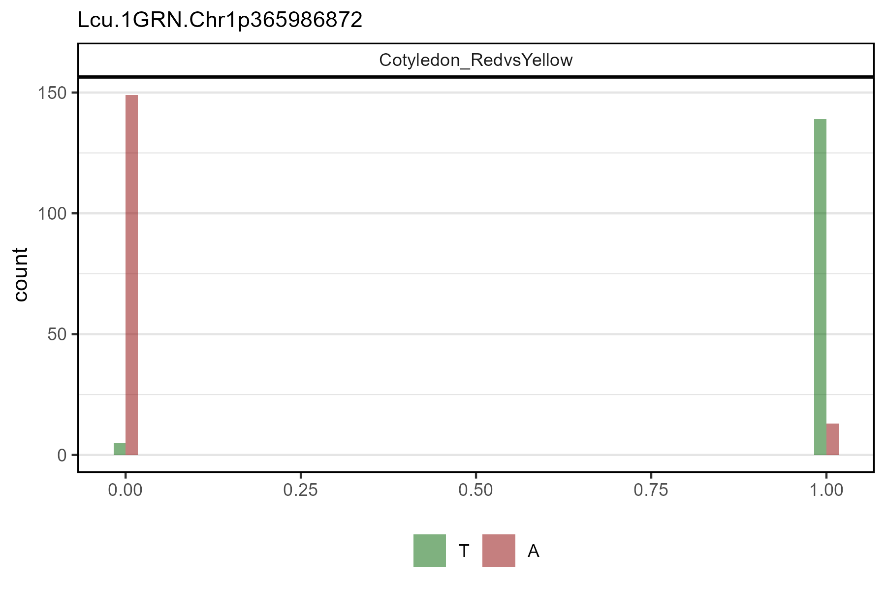
Density
# Plot
mp <- gg_Marker_Bar(
  # Genotype data
  xG = myG,
  # Phenotype data
  xY = myY,
  # Select traits to plot
  traits = "DTF_Sask_2017",
  # Select markers to plot
  markers = "Lcu.1GRN.Chr6p3269280",
  # Select marker colors
  marker.colors = c("darkorange3", "steelblue"),
  # Choose what should be plotted
  plot.histogram = F,
  plot.density = T )
# Save
ggsave("figures/gg_Marker_Bar_03.png",
       mp, width = 6, height = 4)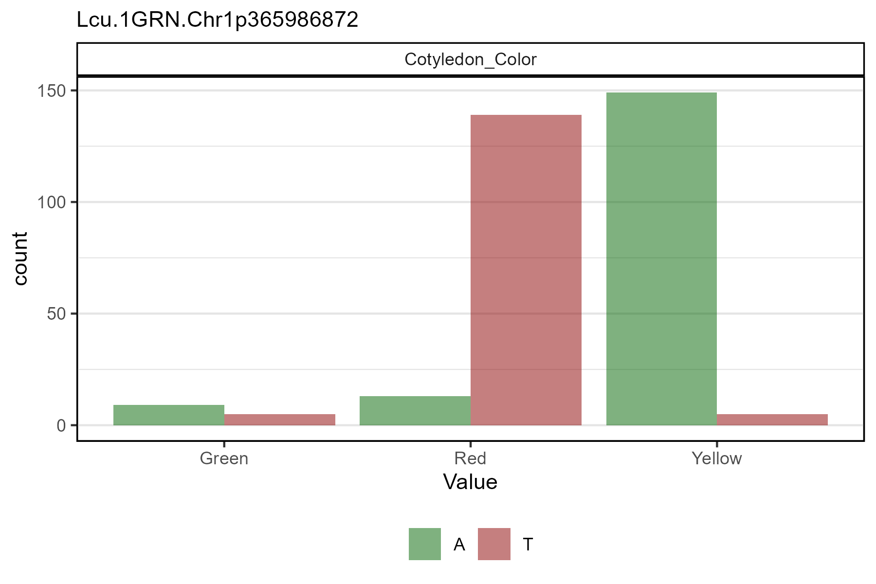
Multiple markers, multiple traits
# Plot
mp <- gg_Marker_Bar(
  # Genotype data
  xG = myG,
  # Phenotype data
  xY = myY,
  # Select traits to plot
  traits = c("DTF_Nepal_2017", "DTF_Sask_2017"),
  # Select markers to plot
  markers = c("Lcu.1GRN.Chr2p44545877", "Lcu.1GRN.Chr5p1658484") )
# Save
ggsave("figures/gg_Marker_Bar_04.png",
       mp, width = 8, height = 4 )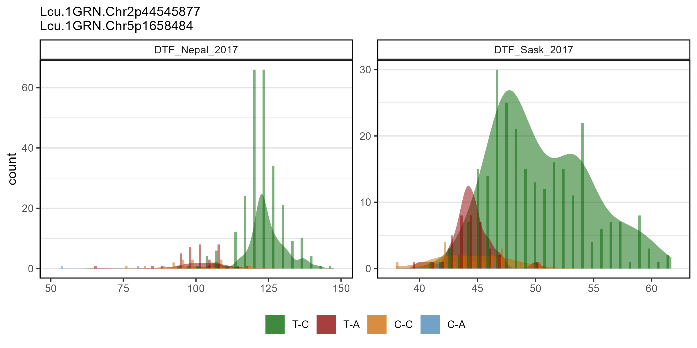
Factor data
Numeric format
# Plot
mp <- gg_Marker_Bar(
  # Genotype data
  xG = myG,
  # Phenotype data
  xY = myY,
  # Select traits to plot
  traits = "Cotyledon_RedvsYellow",
  # Select markers to plot
  markers = "Lcu.1GRN.Chr1p365986872",
  # Select marker colors
  marker.colors = c("darkred", "darkgoldenrod2"),
  # Choose what should be plotted
  plot.histogram = T,
  plot.density = F )
# Save
ggsave("figures/gg_Marker_Bar_05.png",
       mp, width = 6, height = 4 )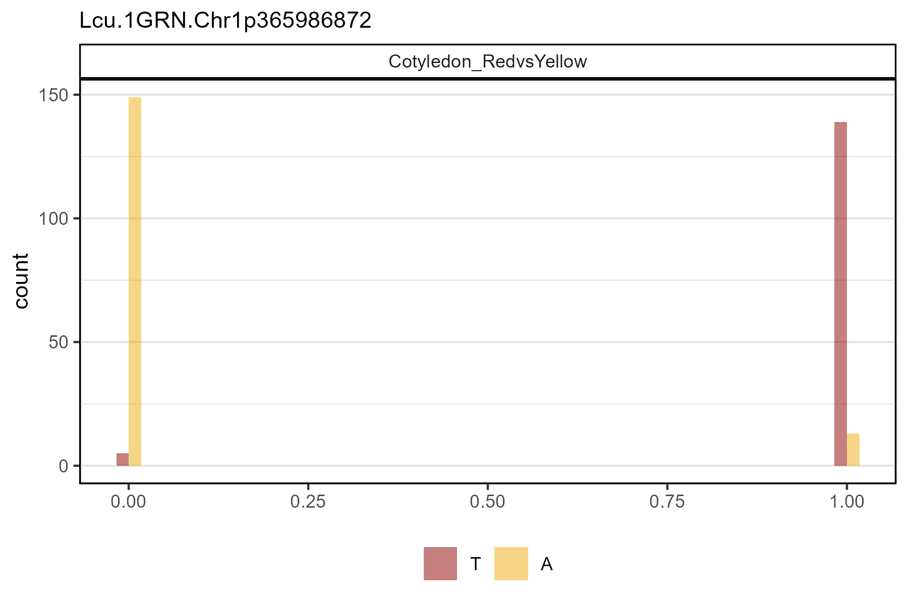
Factor format
# Plot
mp <- gg_Marker_Bar(
  # Genotype data
  xG = myG,
  # Phenotype data
  xY = myY,
  # Select traits to plot
  traits = "Cotyledon_Color",
  # Select markers to plot
  markers = "Lcu.1GRN.Chr1p365986872",
  # Select marker colors
  marker.colors = c("darkred", "darkgoldenrod2", "darkgreen"),
  # Choose what should be plotted
  plot.histogram = T,
  plot.density = F )
# Save
ggsave("figures/gg_Marker_Bar_06.png",
       mp, width = 6, height = 4 )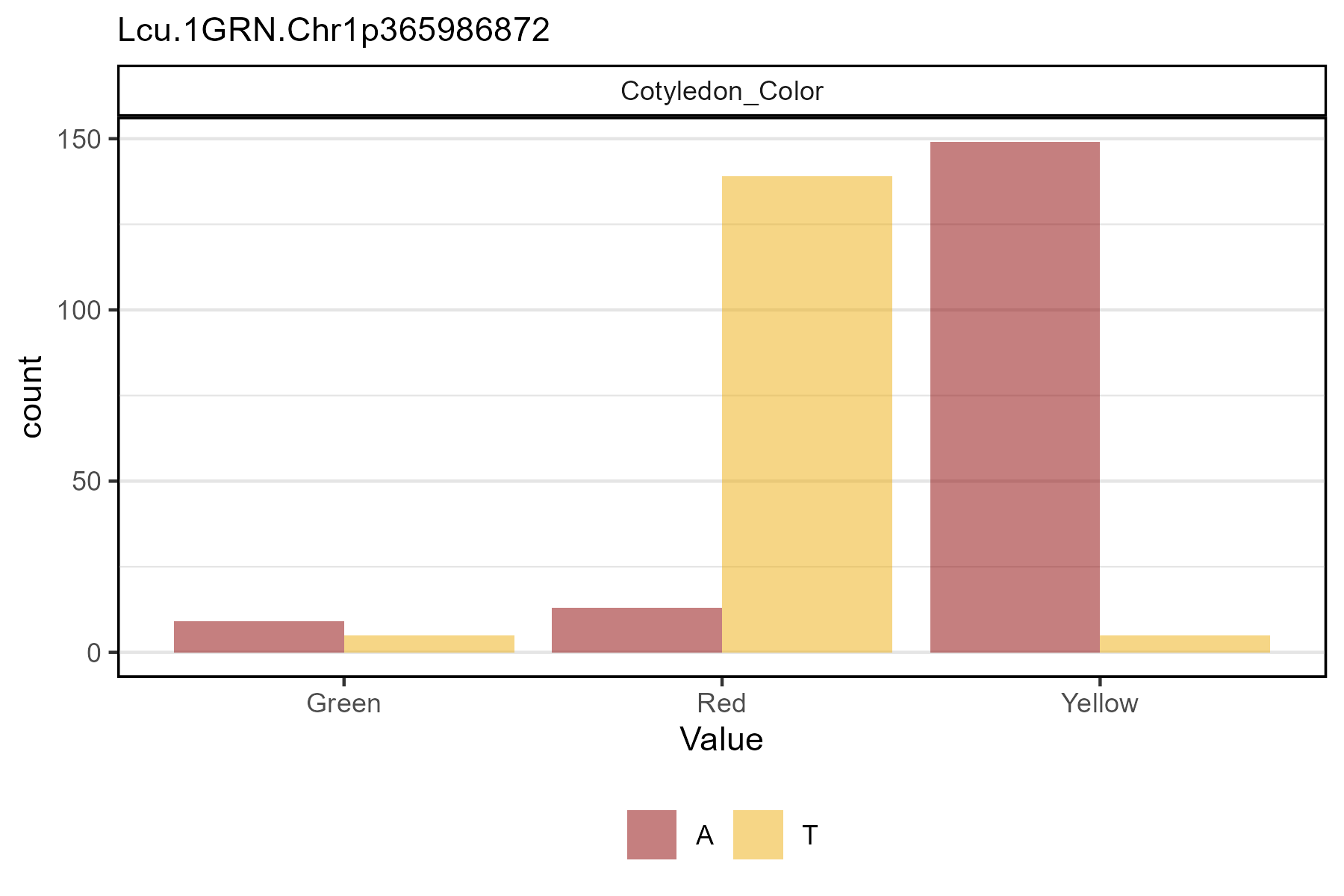
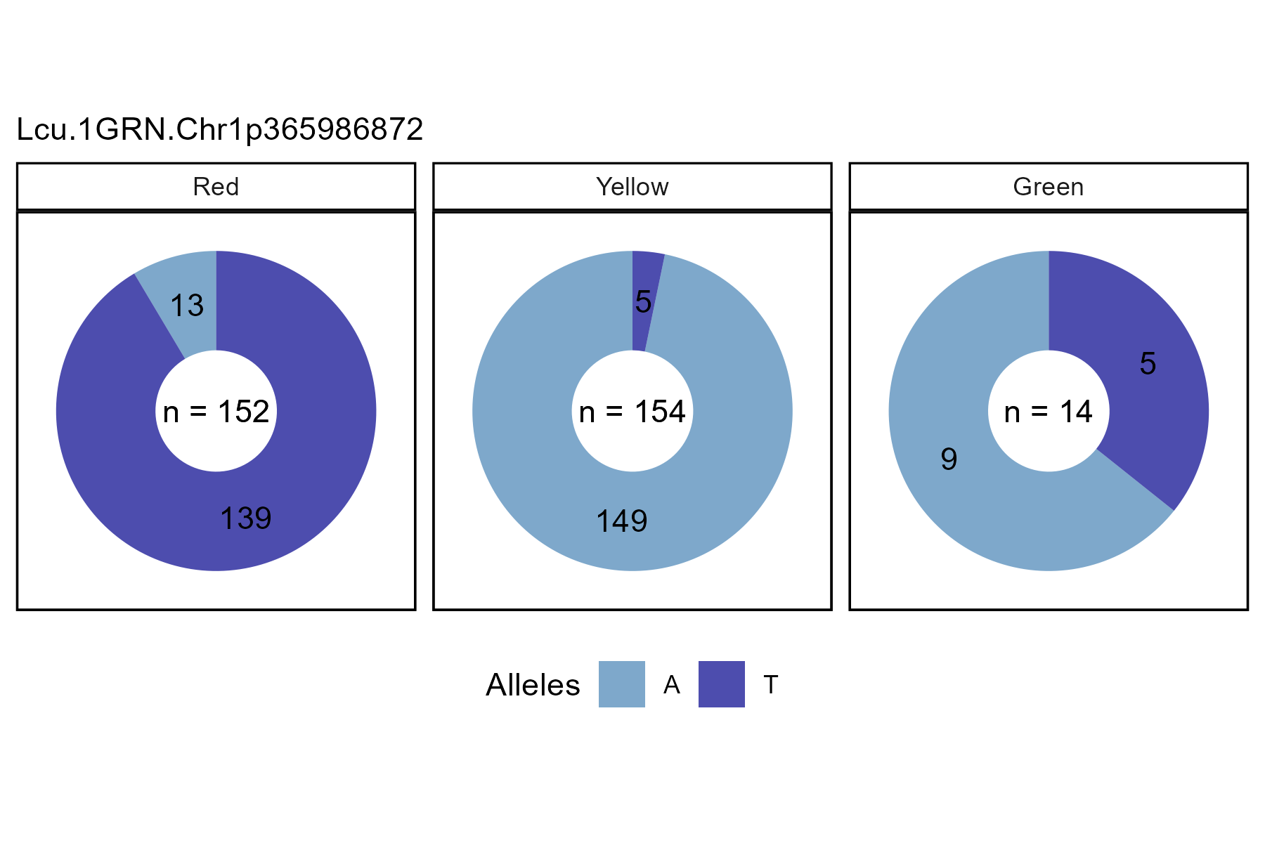
gg_Marker_Pie
# Plot
mp <- gg_Marker_Pie(
  # Genotype data
  xG = myG,
  # Phenotype data
  xY = myY,
  # Select traits to plot
  trait = "Cotyledon_Color",
  # Select markers to plot
  markers = "Lcu.1GRN.Chr1p365986872",
  # Select marker colors
  marker.colors = c("darkred", "darkgoldenrod2", "darkgreen") )
# Save
ggsave("figures/gg_Marker_Pie_01.png",
       mp, width = 6, height = 4 )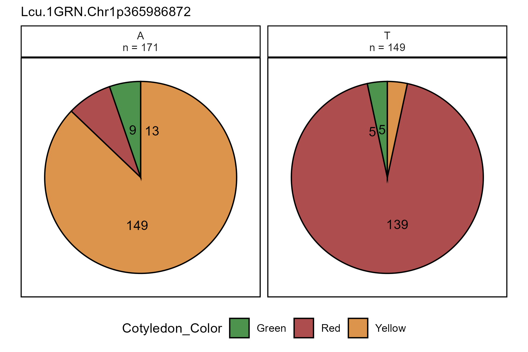
# Plot
mp <- gg_Marker_Pie(
  # Genotype data
  xG = myG,
  # Phenotype data
  xY = myY,
  # Select traits to plot
  trait = "Cotyledon_Color",
  # Select markers to plot
  markers = "Lcu.1GRN.Chr1p365986872",
  # Select marker colors
  marker.colors = c("steelblue", "darkblue"),
  # Make pies of each trait instead of each marker
  groupByTrait = T)
# Save
ggsave("figures/gg_Marker_Pie_02.png",
       mp, width = 6, height = 4 )