The function gg_Marker_Bar() creates marker plots with
your myY and myG GWAS input files.
Load data
Note:
header = T
# Load genotype file (note: header = T)
myG <- read.csv("Data/gwaspr_myG_hmp.csv", header = T)
# Load phenotype file
myY <- read.csv("Data/gwaspr_myY.csv")
Single marker, single trait
Specifying traits and markers along with
your genotype and phenotype data as xG and xY
is needed to create marker plots.
# Plot
mp <- gg_Marker_Bar(
  # Genotype data
  xG = myG,
  # Phenotype data
  xY = myY,
  # Select traits to plot
  traits = "DTF_Sask_2017",
  # Select markers to plot
  markers = "Lcu.1GRN.Chr6p3269280" )
# Save
ggsave("figures/gg_Marker_Bar_01.png",
       mp, width = 6, height = 4 )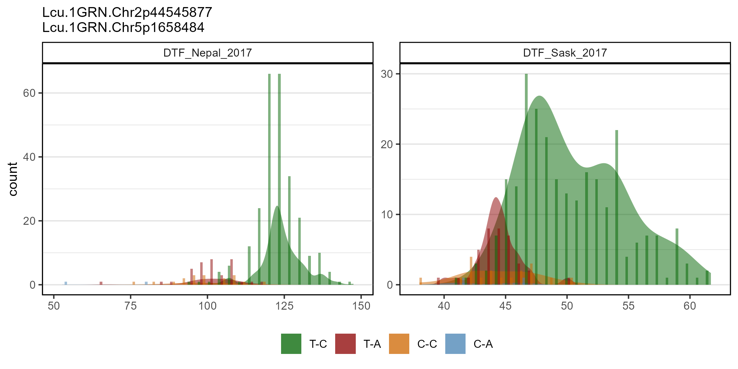
All options
gg_Marker_Bar() contains a number of different options
for customizing the marker plots.
# Prep data
markers <- c("Lcu.1GRN.Chr6p3269280")
# Plot
mp <- gg_Marker_Bar(
  xG = myG,
  xY = myY,
  traits = "DTF_Sask_2017",
  markers = markers,
  marker.colors = gwaspr_Colors,
  remove.hets = T,
  remove.N = T,
  plot.histogram = T,
  plot.density = T,
  plot.counts = T,
  ncol = NULL,
  line.color = F,
  title = NULL,
  subtitle = paste(markers, collapse = "\n"),
  asfactor = F)
# Save
ggsave("figures/gg_Marker_Bar_02.png",
       mp, width = 6, height = 4 )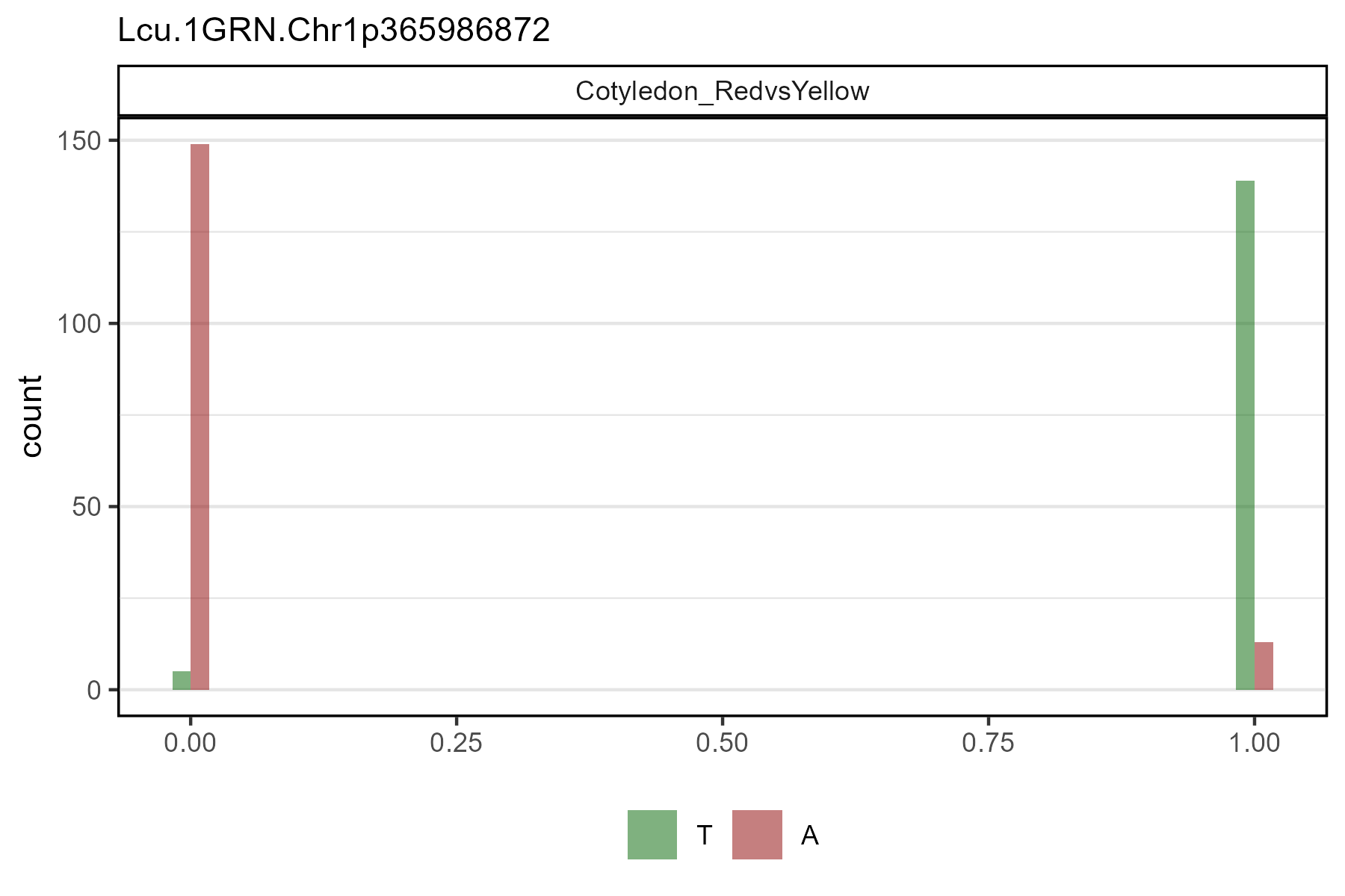
Multiple markers, multiple traits
# Plot
mp <- gg_Marker_Bar(
  # Genotype data
  xG = myG,
  # Phenotype data
  xY = myY,
  # Select traits to plot
  traits = c("DTF_Nepal_2017", "DTF_Sask_2017"),
  # Select markers to plot
  markers = c("Lcu.1GRN.Chr2p44545877", "Lcu.1GRN.Chr5p1658484") )
# Save
ggsave("figures/gg_Marker_Bar_03.png",
       mp, width = 8, height = 4 )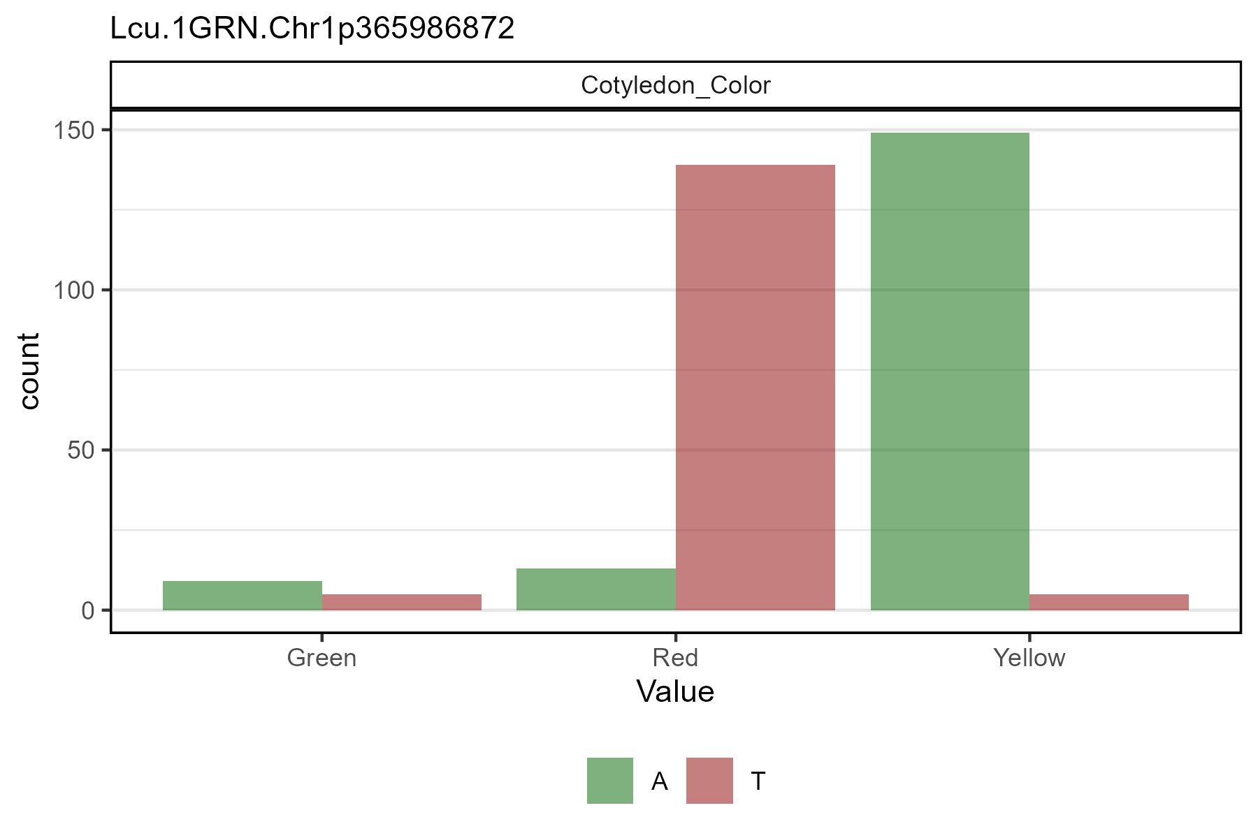
Histogram
# Plot
mp <- gg_Marker_Bar(
  # Genotype data
  xG = myG,
  # Phenotype data
  xY = myY,
  # Select traits to plot
  traits = "DTF_Sask_2017",
  # Select markers to plot
  markers = "Lcu.1GRN.Chr6p3269280",
  # Select marker colors
  marker.colors = c("darkorange3", "steelblue", "darkblue"),
  # Choose what should be plotted
  plot.histogram = T,
  plot.density = F )
# Save
ggsave("figures/gg_Marker_Bar_04.png",
       mp, width = 6, height = 4 )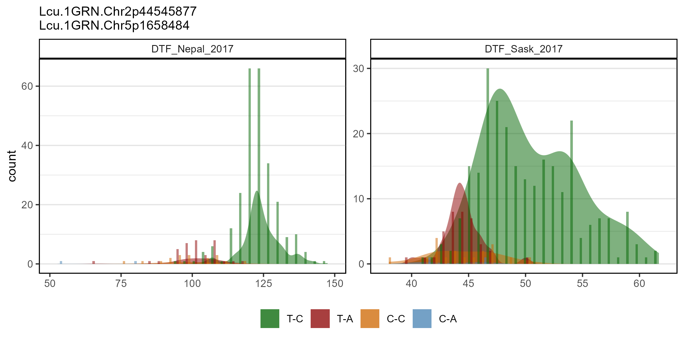
Density
# Plot
mp <- gg_Marker_Bar(
  # Genotype data
  xG = myG,
  # Phenotype data
  xY = myY,
  # Select traits to plot
  traits = "DTF_Sask_2017",
  # Select markers to plot
  markers = "Lcu.1GRN.Chr6p3269280",
  # Select marker colors
  marker.colors = c("darkorange3", "steelblue", "darkblue"),
  # Choose what should be plotted
  plot.histogram = F,
  plot.density = T )
# Save
ggsave("figures/gg_Marker_Bar_05.png",
       mp, width = 6, height = 4)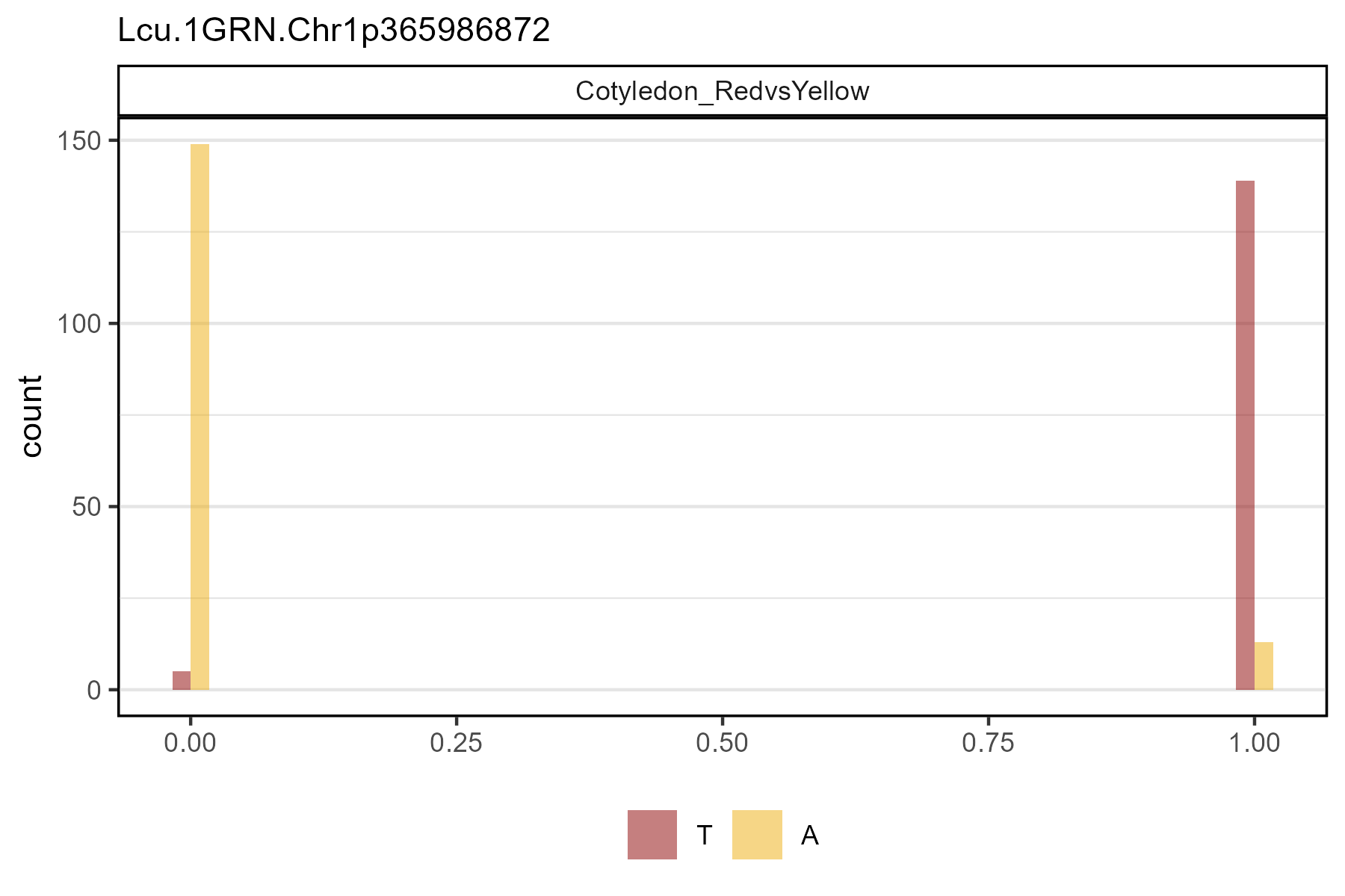
Factor data
Numeric format
# Plot
mp <- gg_Marker_Bar(
  # Genotype data
  xG = myG,
  # Phenotype data
  xY = myY,
  # Select traits to plot
  traits = "Cot_RvY",
  # Select markers to plot
  markers = "Lcu.1GRN.Chr1p365986872",
  # Select marker colors
  marker.colors = c("darkorange3", "steelblue", "darkblue"),
  # Choose what should be plotted
  plot.histogram = T,
  plot.density = F )
# Save
ggsave("figures/gg_Marker_Bar_06.png",
       mp, width = 6, height = 4 )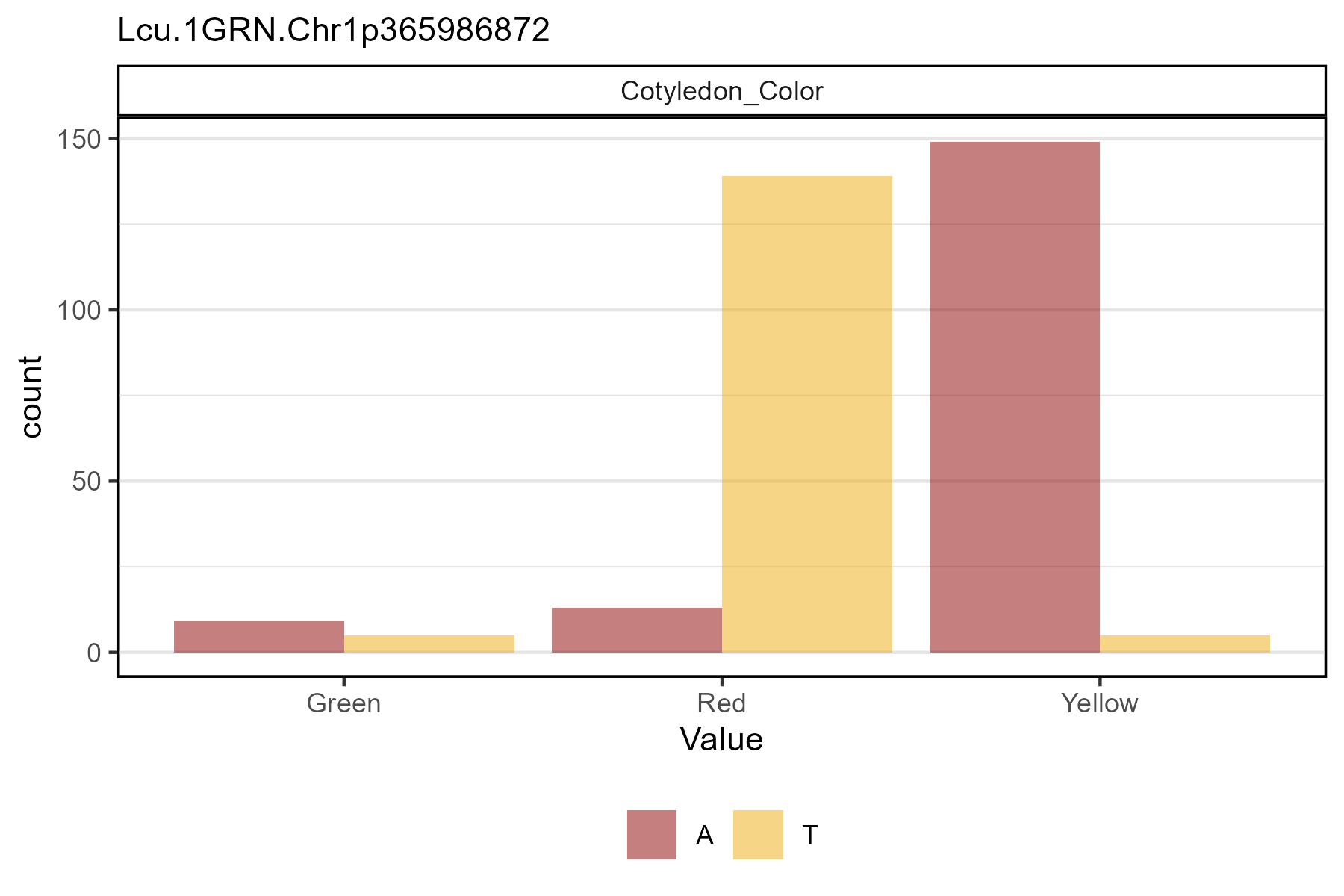
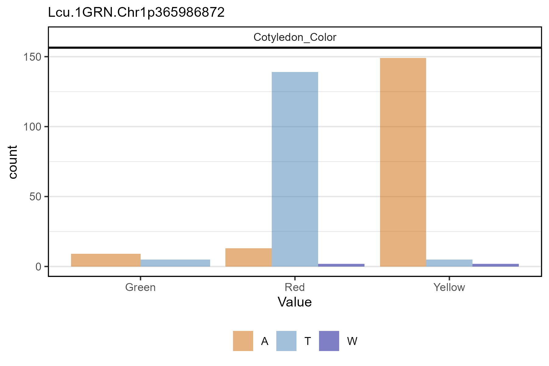
Factor format
# Plot
mp <- gg_Marker_Bar(
  # Genotype data
  xG = myG,
  # Phenotype data
  xY = myY,
  # Select traits to plot
  traits = "Cotyledon_Color",
  # Select markers to plot
  markers = "Lcu.1GRN.Chr1p365986872",
  # Select marker colors
  marker.colors = c("darkorange3", "steelblue", "darkblue"),
  # Choose what should be plotted
  plot.histogram = T,
  plot.density = F )
# Save
ggsave("figures/gg_Marker_Bar_07.png",
       mp, width = 6, height = 4 )